Shortcut Key for Filter in Excel (Excel Shortcuts)

In this video tutorial, we’re going to have a look at how to use the shortcut key for Filter in Excel.

Let’s start!

Shortcut Key for Filter in Excel

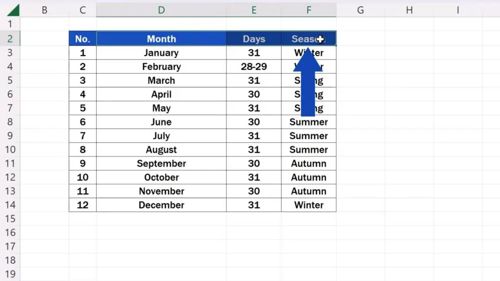
If you need to use Filter in a data table, first, you need to select the headers of the columns in which you’re planning to sort data. Here, we’re going to select the headers Month, Days, and Season.

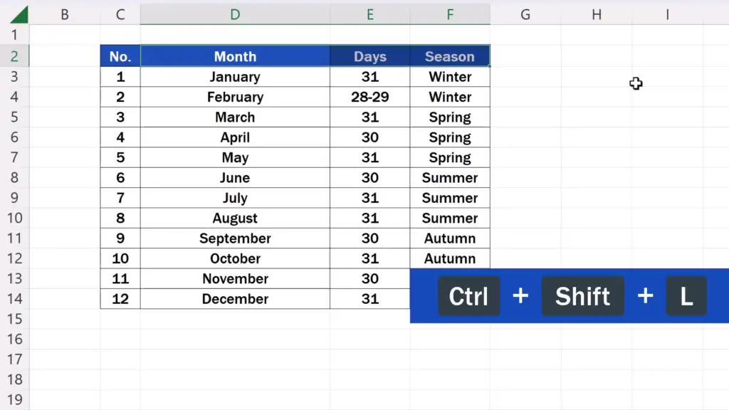
Then, use the shortcut key Control, Shift and L.

And that’s all it takes!

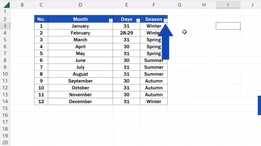
You’ll immediately see these drop-down arrow buttons through which you can conveniently sort and filter data.

Shortcut Key for Removing the Filter in Excel

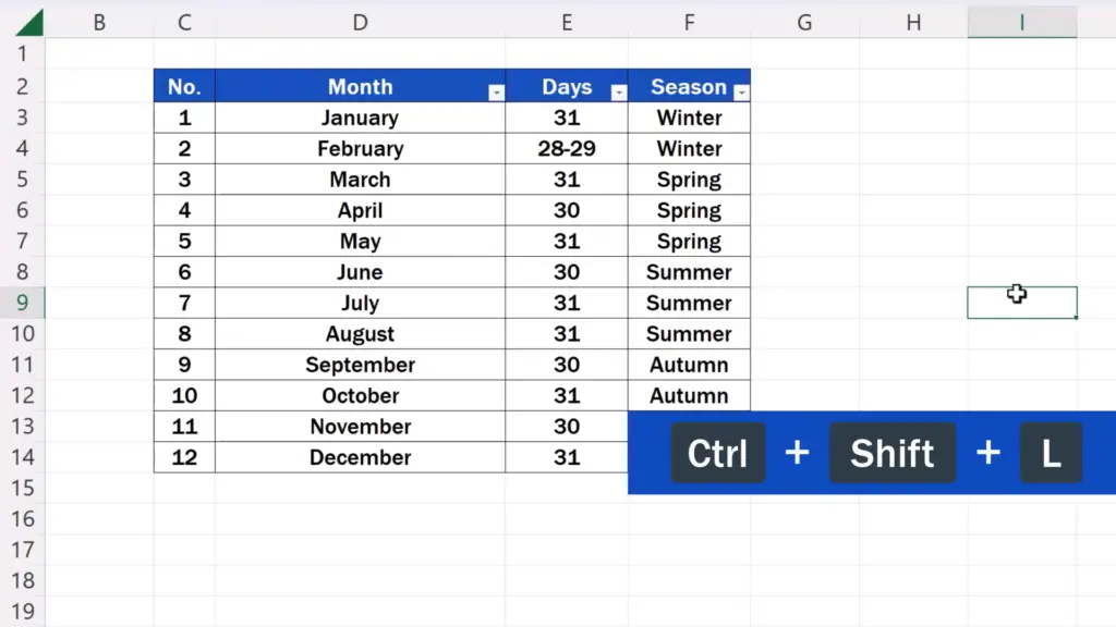
And if you need to remove Filter, just press the shortcut key Control, Shift and L again. The filter’s gone right away!

For advice on other useful Excel Shortcuts, see more tutorials by EasyClick Academy! The links to the tutorials are in the list below.

Don’t miss out a great opportunity to learn:

• Shortcut Key to Insert Rows in Excel (Excel Shortcuts)
• How to Create Filter in Excel
• How to Clear or Remove Filter in Excel

If you found this tutorial helpful, give us a like and watch other tutorials by EasyClick Academy. Learn how to use Excel in a quick and easy way!

Is this your first time on EasyClick? We’ll be more than happy to welcome you in our online community. Hit that Subscribe button and join the EasyClickers!

Thanks for watching and I’ll see you in the next tutorial!