How to Use the VLOOKUP Function in Excel (Step by Step)

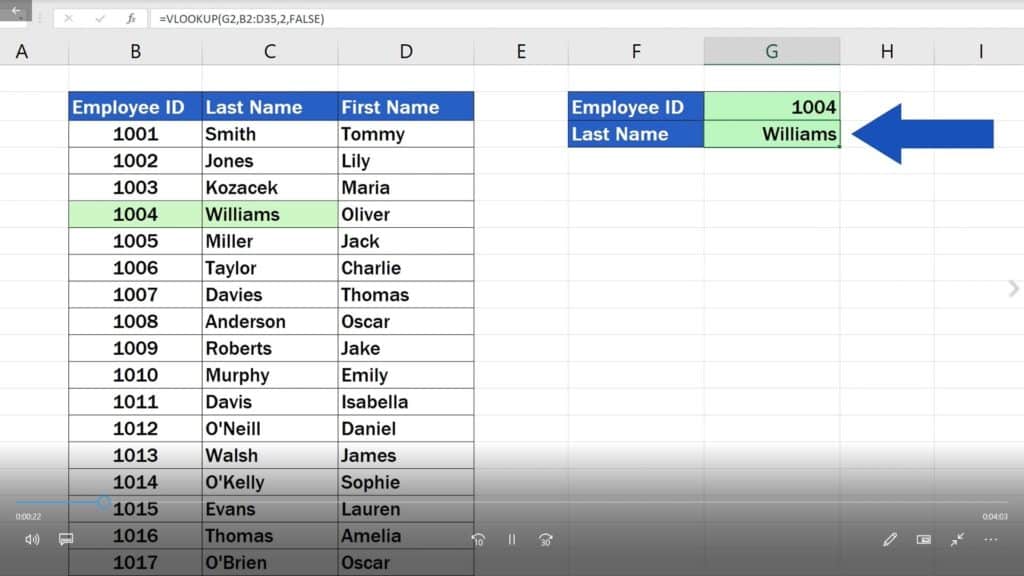
This tutorial offers a detailed description of how to use VLOOKUP in Excel. This function works like a phone book. Based on the information you know Excel will look up the details you don’t know and need to find out in a data table. For example, you know what an employee’s ID is and based on that, you can look up the employee’s family name.

If you’re curious how to use VLOOKUP, let’s go through it, step by step, together!

Would you rather watch this tutorial? Click the play button below!

The VLOOKUP function is particularly useful if there’s a great deal of data stored in the data table in which you regularly need to carry out the search for certain information.

Today, we’re gonna have a look at how to look up the last name of an employee based on their ID.

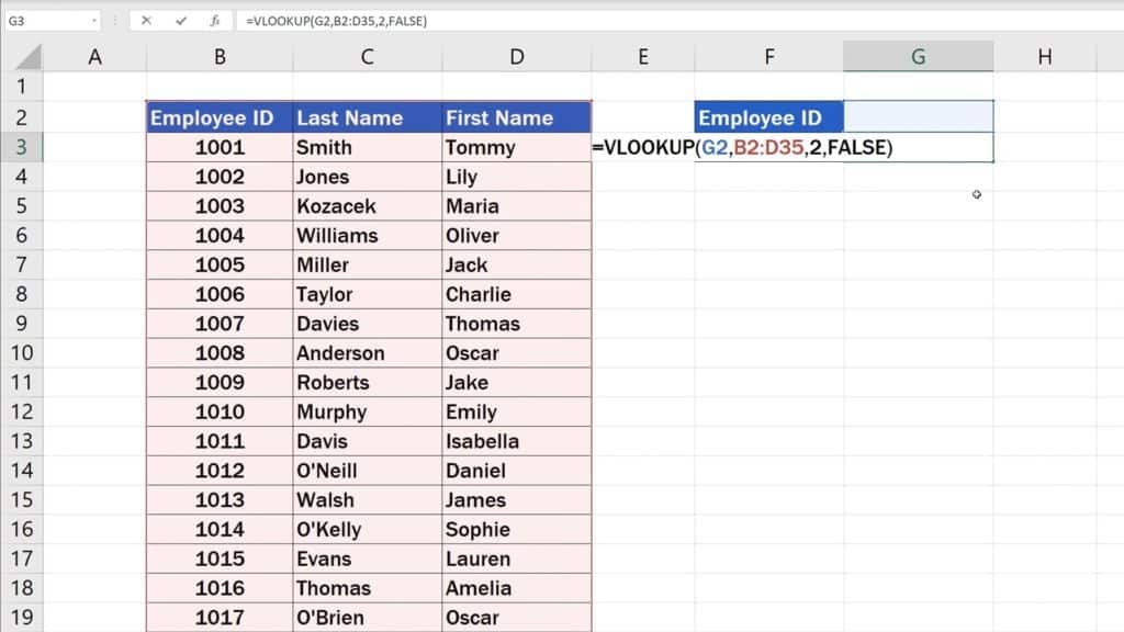
To begin, select the cell where you want the search result to appear. In this case, it will be the cell next to ‘Last Name’. Type in the equal sign, then ‘VLOOKUP’, and select the suggested function. To make the function work, we’ll need to enter some more details.

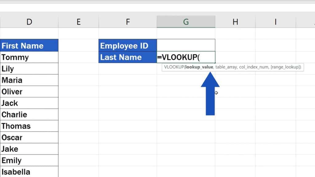
The VLOOKUP function – The Details Needed to To Make the Function Work

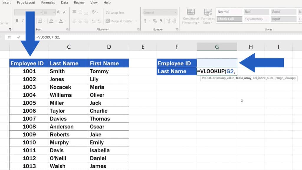
First, we need to state according to what Excel should look for the piece of information we need to find, which will be ‘Employee ID’. The Employee ID will be entered in the cell G2, so we’ll click and select that cell to include it in the formula and enter a comma.

The next piece of information Excel needs is the area which will be searched. This area must include both details ‘Employee ID’ as well as ‘Last Name’.

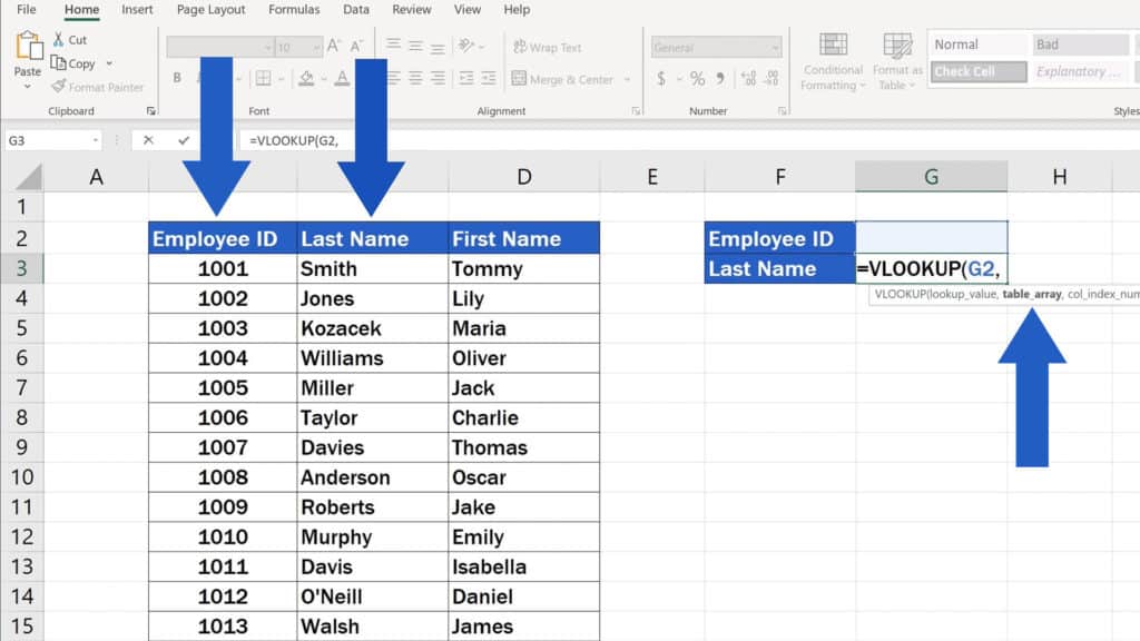
Here we need to mention that VLOOKUP works with the information thoroughly organised. The function looks to the right, which means that if you want it to work, the information based on which you carry out your search must be located to the left of the information you want to find.

This means that the Employee ID column must be on the left, and the Last Name column needs to appear on the right in the table.

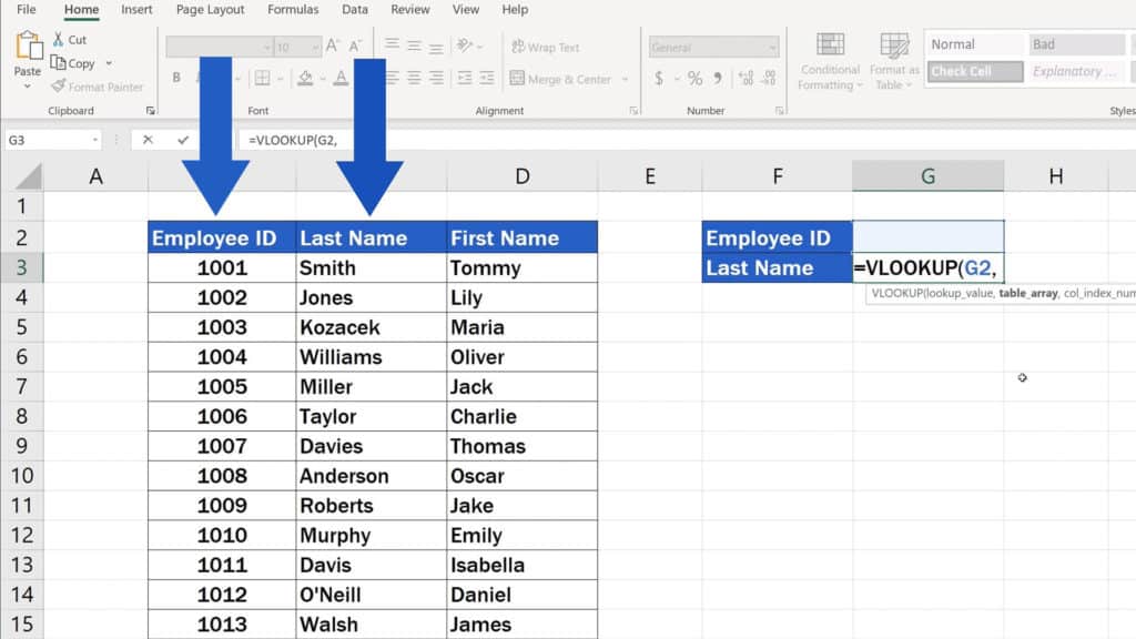
To select the area of search, you can mark the whole table, add a comma and we’ll move on to the next step.

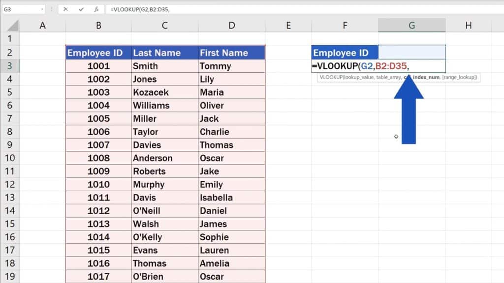
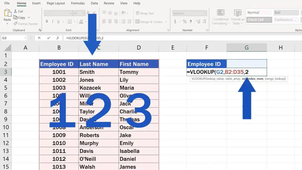
What Excel needs here is the number of the column that contains the information we want to retrieve. The column numbering in the selected area is standard – 1, 2 and 3. Since we want to look up the last name, and this information is stored in the second column, we’ll type in ‘2’. Enter a comma again, and we’ve got the last bit ahead of us.

The Last Part of the Formula – True or False Function

In the last part, the formula requires one of the words ‘True’ or ‘False’. If you enter ‘True’, Excel will look for an approximate match. That is the default option. But if you are looking for the exact match, you need to type in ‘False’.

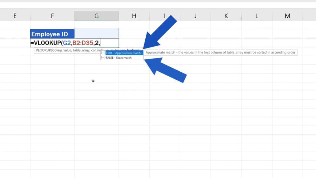
In this case, we want Excel to look up the employee’s family name based on the exact match of the employee’s ID, so we’ll use ‘False’ here. Click on ‘Enter’ and the job’s done!

The Examples of How the VLOOKUP Function Works in Excel

The VLOOKUP function is complete and correct, but we didn’t enter any Employee ID. That’s why there’s no result in the field ‘Last Name’ for the time being.

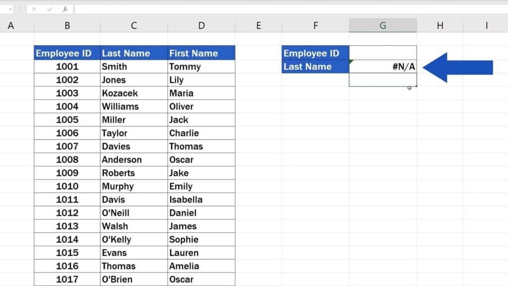
Once we enter an ID, it will look for the exact match of what we entered, and based on it, Excel will provide us with the employee’s family name.

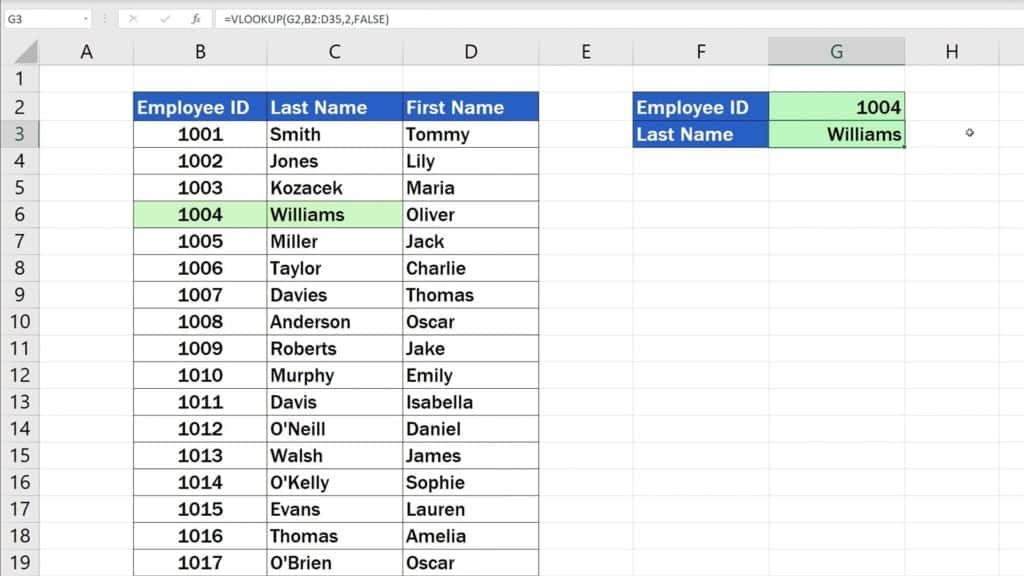
So, if we enter for example ‘1004’, Excel will find for us the Last Name of the employee with the ID 1004, which is, in this case, Williams.

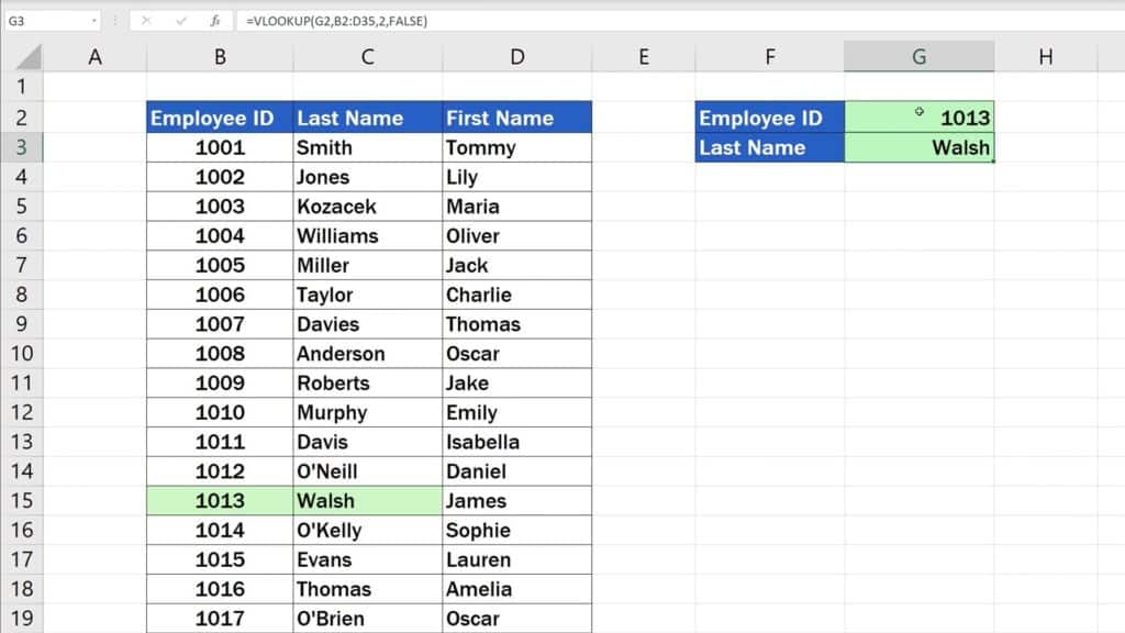
If we type in ‘1013’, Excel will show that the last name of the employee with this ID is Walsh.

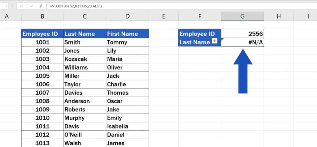
If we enter an ID which is not present in the data table, Excel will not show any valid result.

Well, this was a short video on how to use one of the most favourite functions in Excel – VLOOKUP. More tutorials on other popular functions are listed in the description list below.

Don’t miss out a great opportunity to learn:

• How to Calculate Difference Between Two Dates in Excel
• How to Sum a Column in Excel

If you found this tutorial helpful, give us a like and watch other video tutorials by EasyClick Academy. Learn how to use Excel in a quick and easy way!

Is this your first time on EasyClick? We’ll be more than happy to welcome you in our online community. Hit that Subscribe button and join the EasyClickers!

Thanks for watching and I’ll see you in the next tutorial!