How to Use IF Function in Excel (Step by Step)

IF function comes handy when you need to evaluate a logical condition and quickly find out whether it is true or false.

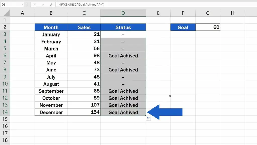
In this tutorial, you’ll see how the function IF helps evaluate whether the sales for a particular month met the goal that had been set. If yes, Excel will display the message ‘Goal Achieved’. If the condition comes out as false, a horizontal stroke will show instead of the message.

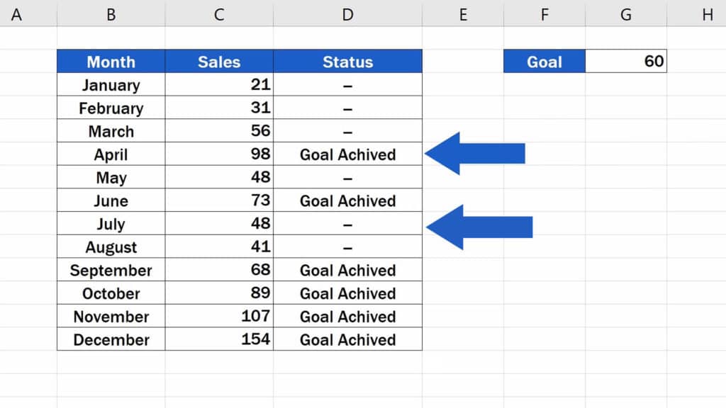
So, how can we use IF Function effectively?

Would you rather watch this tutorial? Click the play button below!

What is the Syntax of the IF Function

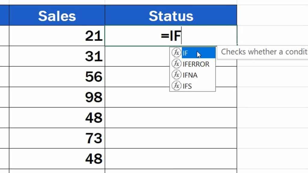
To start, click into the cell which you selected to show the result. We’ll click in the cell D3. Type in the equal sign and right after that, ‘IF’. Excel will offer more functions out of which we select ‘IF’ by clicking on it.

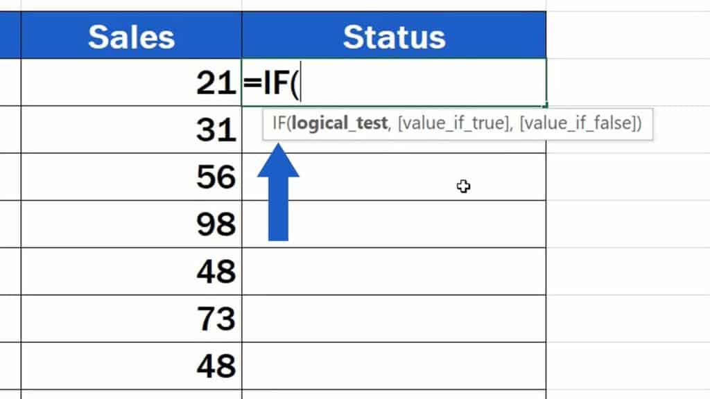
Then you’ll need to add three details – the logical test, which is what Excel evaluates, and two different values – one will be displayed if the logical test result is true, the other if it’s false.

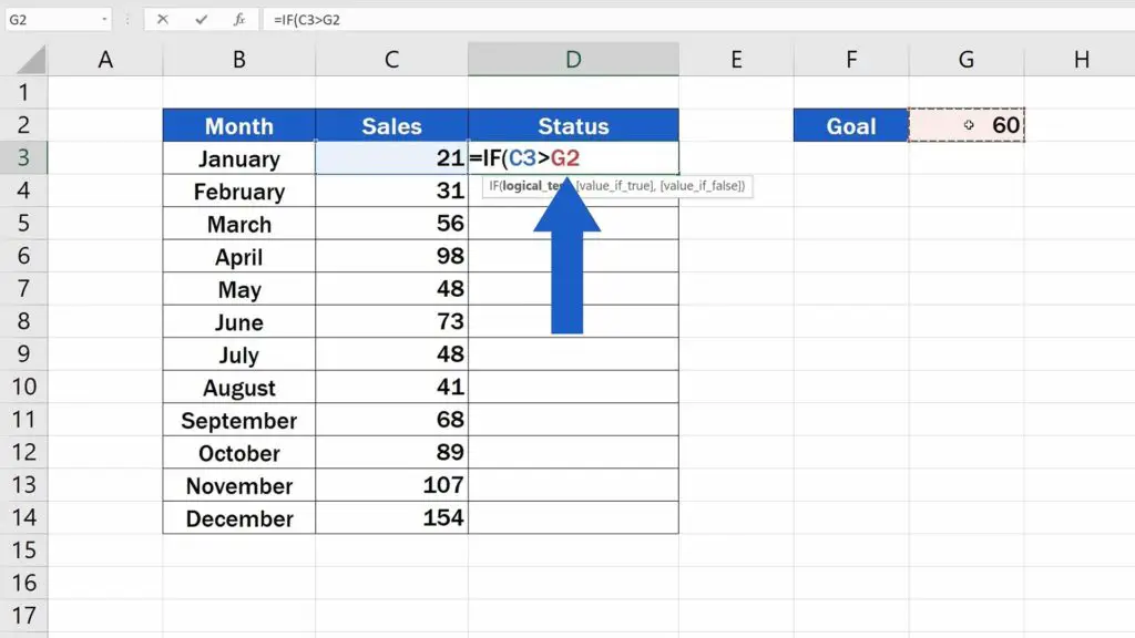
Let’s start with entering the logical test first. In this formula, we’re going to compare whether the sales in this particular month were higher than our goal.

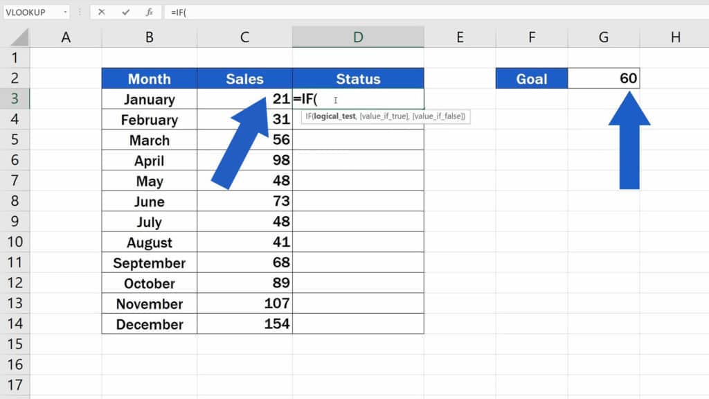
So, we’re trying to find out whether the number in the cell C3 (sales for January) is higher than our goal in the cell G2.

This way you can compare whether something is greater than or less than or equals to something else.

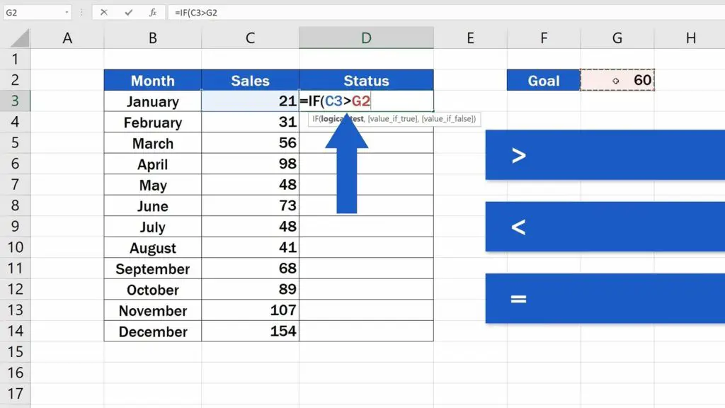
There’s a possibility to nest another IF Function inside the logical test of this IF Function, which allows you to make further, more complex comparisons.

As soon as the logical test has been entered, carry on typing a comma and we’ll move on.

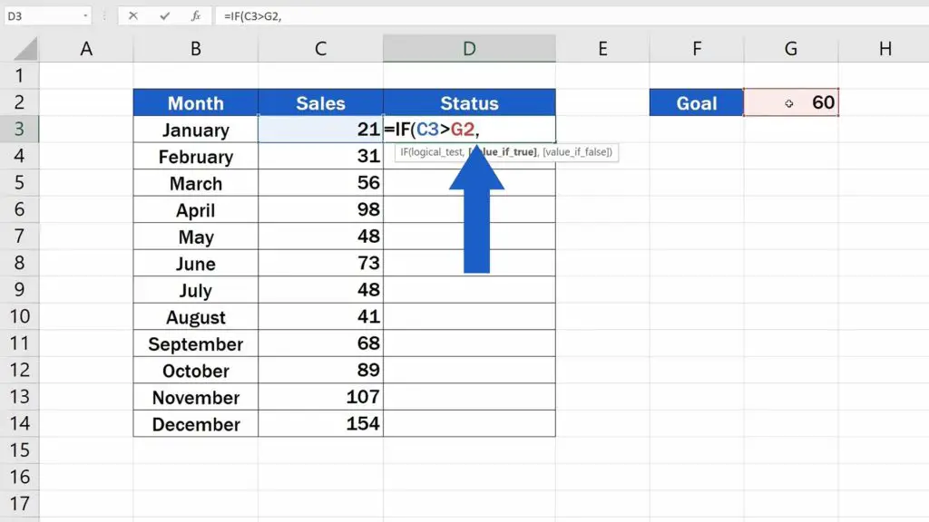
Now, Excel needs a value that will appear as the result if the condition we entered comes out as true. After that we’ll need to enter a value if this condition is evaluated as false.

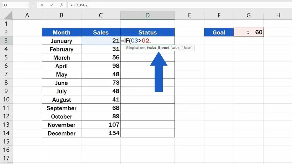
Let’s have a look at the first value, which appears if the condition is evaluated as true. If you want Excel to display a text, in our case the message ‘Goal Achieved’, you need to type it in like this – in quotation marks.

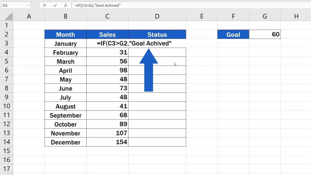
If this first value is a number, we standardly don’t put it in quotation marks. After typing in the message, add a comma.

Now we need to enter the second value, which is the value Excel will show if the condition comes out as false.

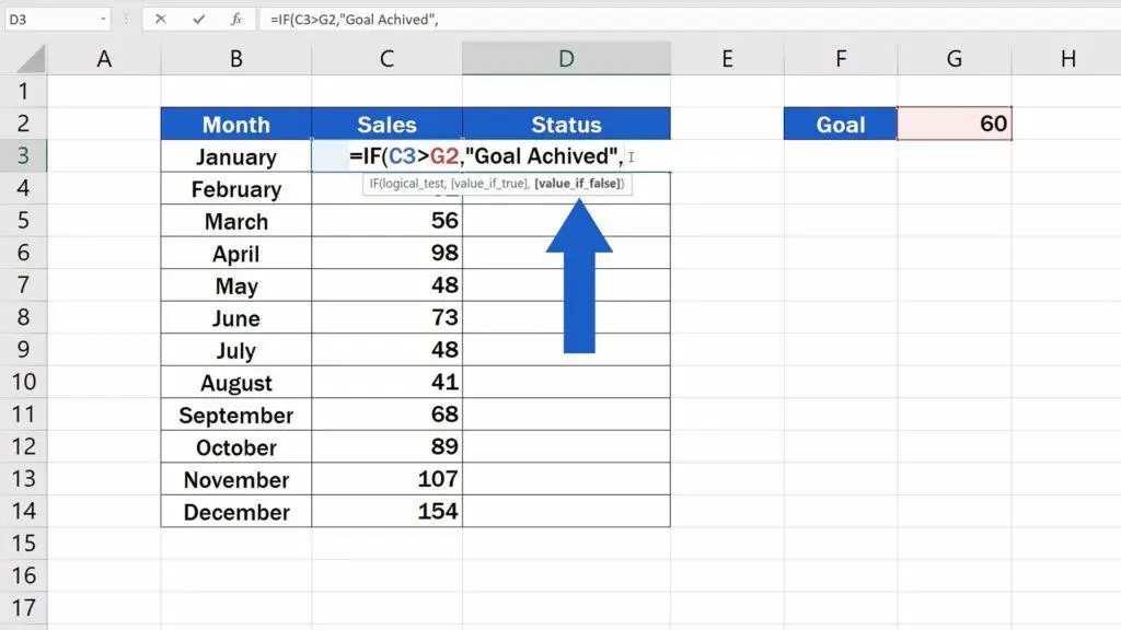
If the sales in this month did not reach our goal, we want Excel to show not a message, but a horizontal stroke, so we’ll enter a dash in quotation marks.

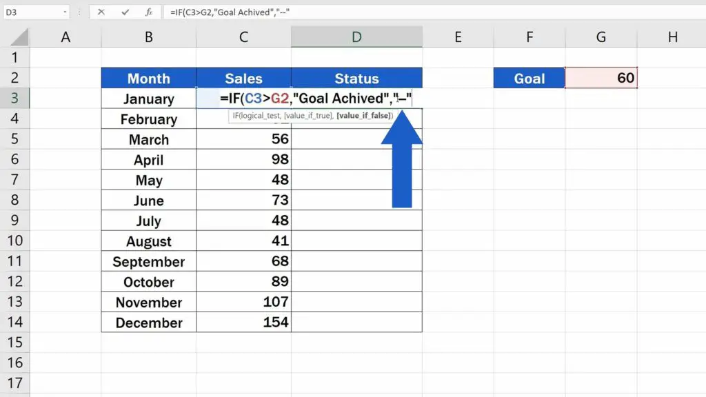
All three necessary details have now been added, so let’s close the brackets and press ‘Enter’. Well done! The function immediately evaluated that in January, we did not meet our goal.

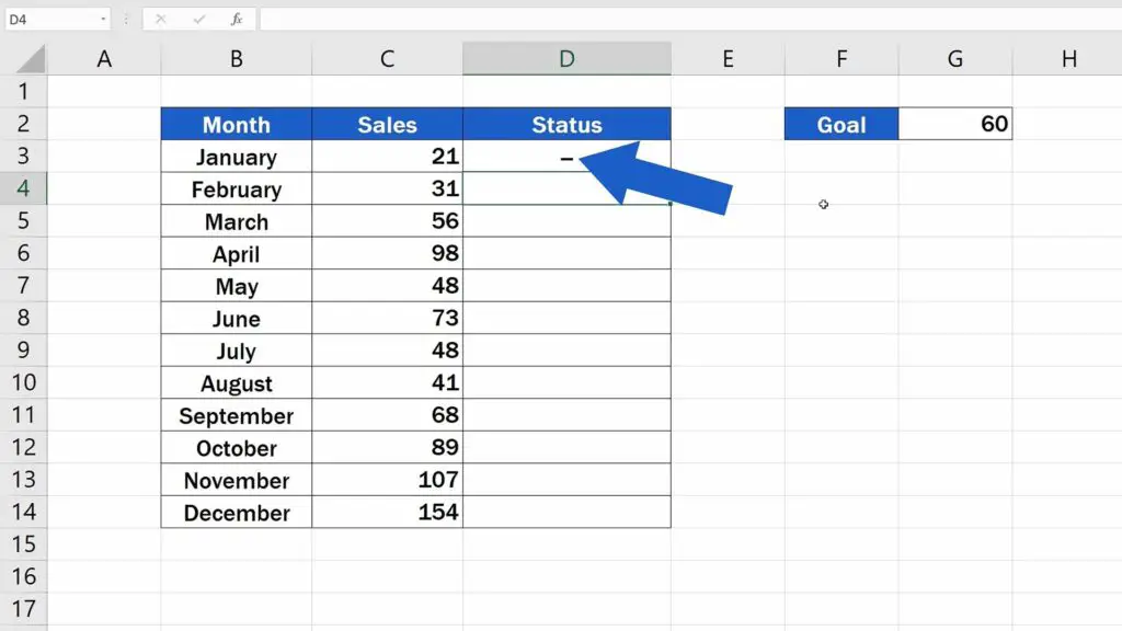
But watch out now!

How to Copy the Function IF to the Rest of the Column

A little complication might appear if you want to copy the function to the rest of the column. Thanks to the little trick we’re about to share with you, it’ll be no problem!

You might’ve guessed correctly that if we want to use the function to evaluate the sales numbers for the rest of the months, we need to copy the function by dragging the bottom left corner of the cell where the function has already been placed.

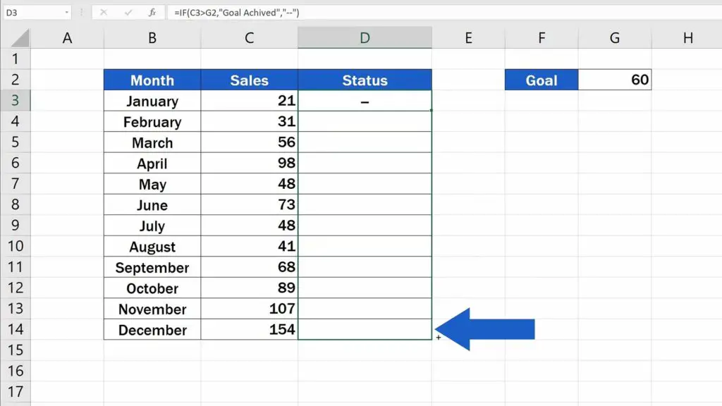
However, the function seems not to be working properly once copied. For example, if you have a look at row 4, the cell reference to the Goal has moved one cell down, to G3. But that cell contains no value. The same happens in row 5, Excel refers to a wrong cell for Goal.

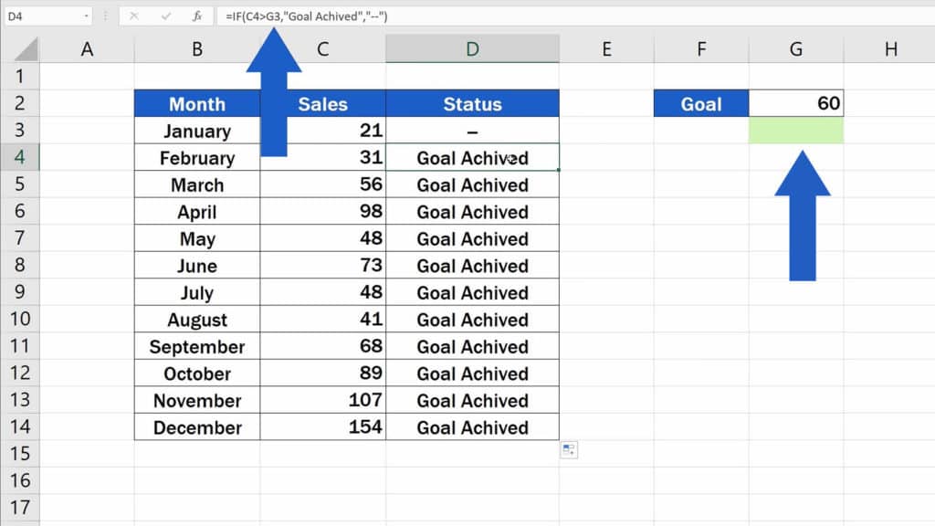
How to fix this?

Have a look at the original formula which was previously copied to the rest of the rows. We need to keep the reference we make here to the Goal fixed. Click into that part of the formula that refers to the cell where the Goal value is stored, which is G2. Now press the F4 key. Some of you might need to hold the Function Key (Fn) while pressing F4.

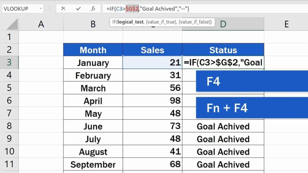
As you can see, two dollar signs appeared, one in front of the letter – this fixes the column – and another one in front of the number – this one fixes the row.

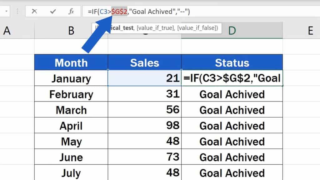
Using these dollar signs makes the reference to a specific cell fixed. In all rows now, the copied formula will use only the cell G2 to calculate the result. This little trick works in all Excel formulas and functions, so you can use it whenever you need!

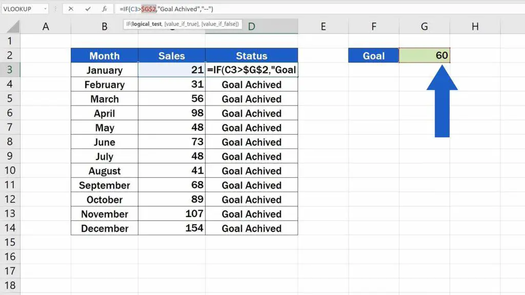
Let’s hit ‘Enter’ again and let’s try to drag the formula down the rest of the cells one more time. And we can see that the function works perfectly now! Each row contains the correct evaluation of the sales numbers against the goal we’ve set.

IF Function is Dynamic

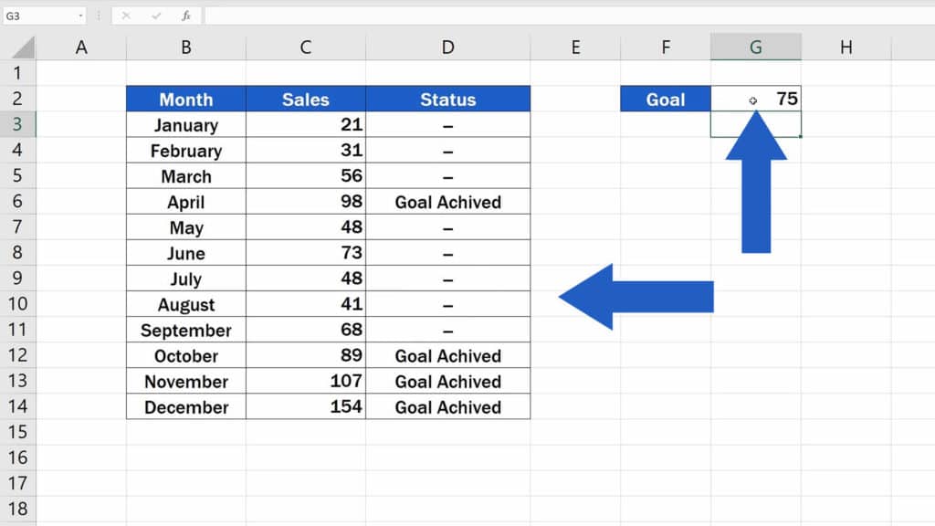
Remember, IF Function is dynamic, which means you don’t need to update the formula if you change the value of the goal in the cell G2. The results in column D will be automatically updated.

To see more ways how you can use the IF functions, check out our tutorial on how to calculate hours worked in Excel (midnight span), where we used the logical test to find out whether the working time spanned midnight. The link to the tutorial can be found in the list below along with tutorials for other popular functions in Excel.

Don’t miss out a great opportunity to learn:

• How to Calculate Hours Worked in Excel (Midnight Span)
• How to Calculate Difference Between Two Dates in Excel
• How to Sum a Column in Excel
• How to Use the VLOOKUP Function in Excel (Step by Step)

If you found this tutorial helpful, give us a like and watch other video tutorials by EasyClick Academy. Learn how to use Excel in a quick and easy way!

Is this your first time on EasyClick? We’ll be more than happy to welcome you in our online community. Hit that Subscribe button and join the EasyClickers!

Thanks for watching and I’ll see you in the next tutorial!