How to Unhide Sheets in Excel

In this tutorial, we’ll carry on with how to unhide hidden Spreadsheets in Excel.

So let’s get into it!

See the video tutorial and transcription below: 

See this video on YouTube:
https://www.youtube.com/watch?v=F5Fq4lnYsHA

Previously, you learned how to hide a sheet in Excel in a quick and simple way.

Now, we’ll have a look at how to revert this step and you’ll also see how you can easily find out how many hidden sheets there are in a workbook and what their names are.

As an example, we’ll use the same table as we did last time. You can notice that the only visible sheet here is the sheet ‘Questionnaire’.

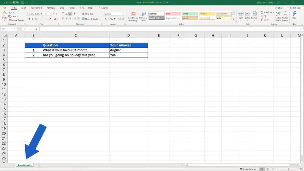
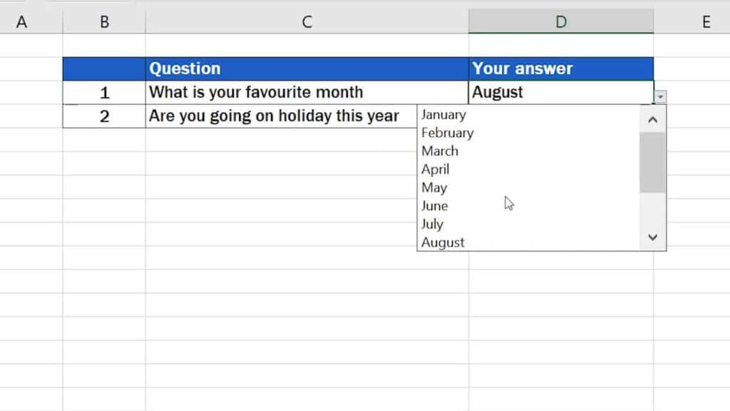
But there is a hidden spreadsheet in the workbook with the list of all months that was used to help us make this drop-down menu.

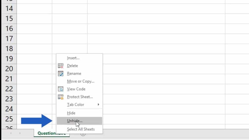
So, if you want to unhide a sheet in a workbook, you’ll need to click on any spreadsheet that is visible. Set the cursor on its name, right-click and select ‘Unhide’.

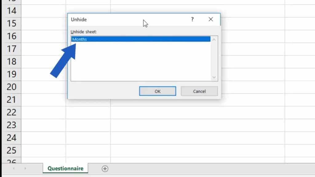
You’ll see a pop-up window where you’ll find the list of all spreadsheets currently hidden in the workbook. In this case, only one spreadsheet is hidden, the spreadsheet called ‘Months’.

What to Do if There Is More then One Hidden Sheet

If there were more, you’d need to select and click on the one you want to unhide. Then click on OK.

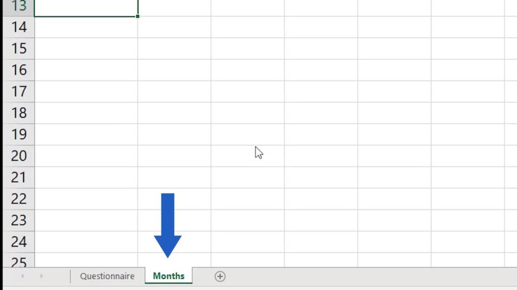
Great! The spreadsheet ‘Months’ with the source data for our drop-down list is visible again on the bar below!

Are you wondering:

• How to Hide Sheets in Excel
• How to Insert Sheet in Excel
• How to Delete Sheet in Excel
• How to Rename Sheet in Excel

If you found this tutorial helpful, watch other video tutorials by EasyClick Academy. Learn how to use Excel in a quick and easy way!

Is this your first time on EasyClick? We’ll be more than happy to welcome you in our online community. Hit that Subscribe button on our YouTube channel and join the EasyClickers!

See you in the next tutorial!