How to Unhide Columns in Excel

In this tutorial, I’ll show you some easy steps on how to unhide columns in Excel, which will show the data in these columns.

So, let’s have a look at it!

See the video tutorial and transcription below: 

See this video on YouTube:  
https://www.youtube.com/watch?v=qPZ-fawdp84

In the previous tutorial, we learned how to hide columns in Excel. Now, we’ll learn how to unhide them.

Generally, it’s quite easy to spot the hidden columns in a spreadsheet.

How to Spot the Hidden Columns in a Spreadsheet

One way to find them is to look for ‘a double-line’ among the column headings. Skipped letters of the alphabet is another sign how to recognise that some columns have been hidden. Normally, the letters would go A, B, C, D, and so on. In this case, however, we see the column C right next to the column F, which means that the columns D and E have been hidden.

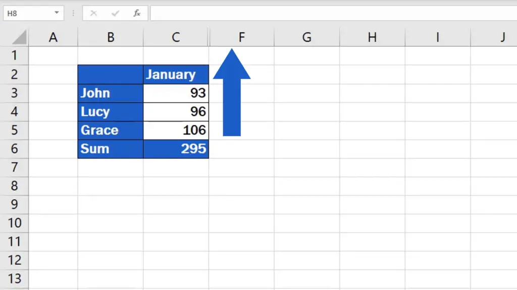
And it’s time to learn two simple ways how to unhide these columns.

Here’s one of them!

The First Way How to Unhide Columns in Excel

First, you’ve got to select the columns you want to unhide. You can do it by selecting one column on the left- and one on the right-hand side of the column or columns you want to unhide. Right-click, find the option Unhide which will make the hidden columns visible again.

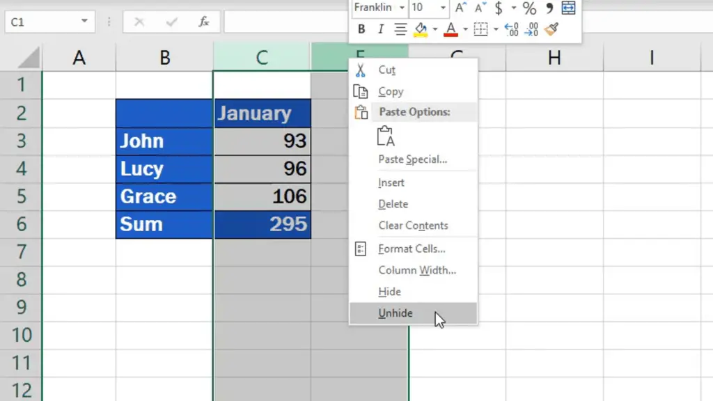
These columns then appear in the table on the screen and if you want to print the sheet out, they will also appear on the printed copy.

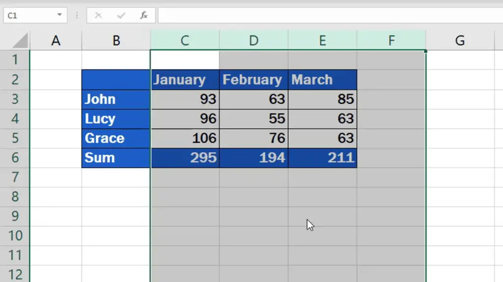
We’ll undo the changes now to have a look at the other way how to unhide columns in Excel.

The Second Way How to Unhide Columns in Excel

Once again we’ll select the columns we want to unhide the same way we did earlier. Go to the Home tab, Cells section, choose the option Format, then option Hide & Unhide from the menu, and we’ll click on Unhide Columns.

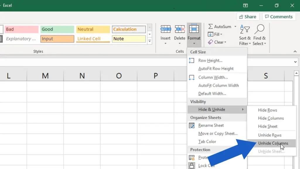
Well done!

Before we wrap it up, I’ve got a couple of handy tips for you.

How to Unhide the Very First Column in Excel

If the column hidden is the column A, which is the very first in the spreadsheet, you’ll need to select the column B first (which is the column on the right), and then highlight the row headings (containing numbers) on the left. This is how you highlight the hidden column A from both sides.

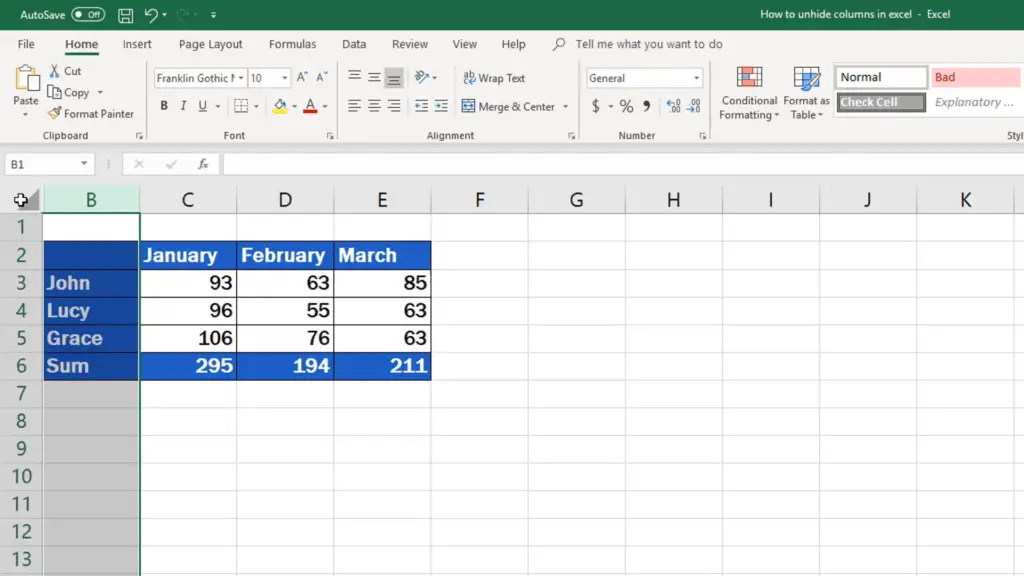
And you can easily unhide it now!

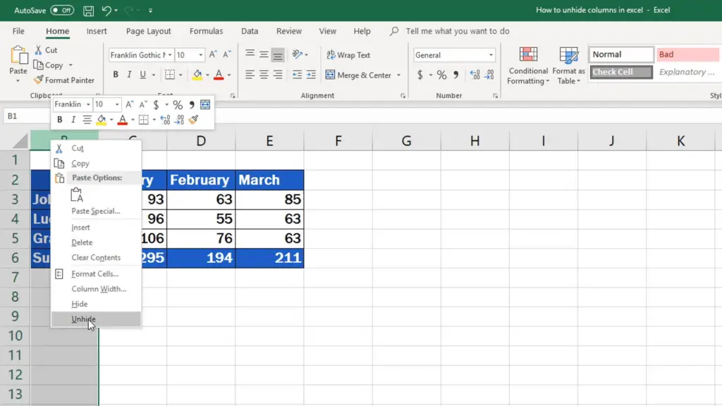
Let’s undo the changes to see the second useful tip.

How to Unhide All Columns in the Whole Spreadsheet

If you want to unhide all columns in the whole spreadsheet, click here, into the top left-hand corner. The whole sheet is now highlighted.

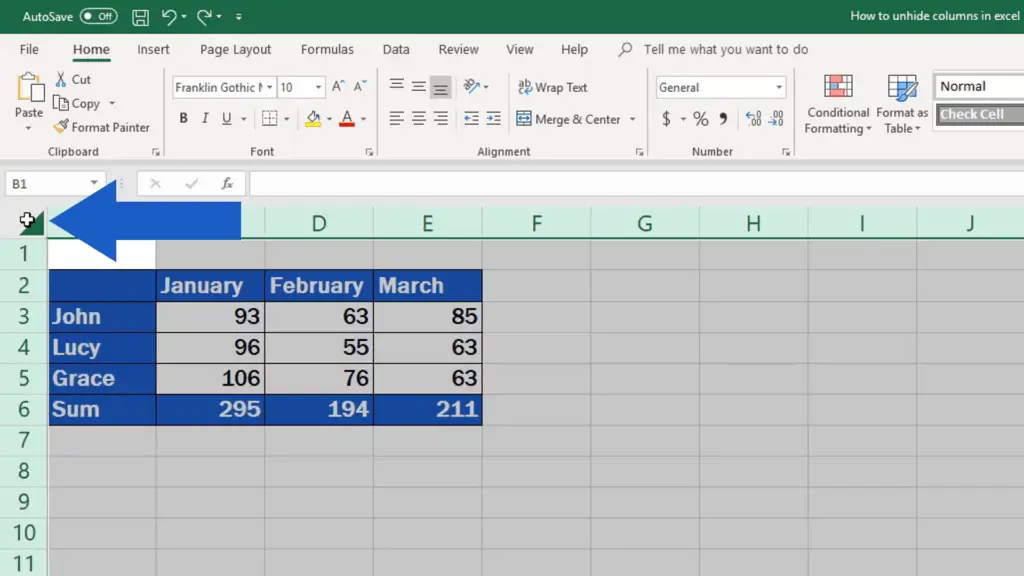
Do the right-click on the column headings part, pick the Unhide option – all columns in the whole spreadsheet will become visible.

Would you like to know:

• How to Hide Columns in Excel
• How to Hide Rows in Excel
• How to Hide Sheets in Excel
• How to Insert Column in Excel

If you’ve found this tutorial helpful, like us and subscribe to receive more videos from EasyClick Academy. Look at more tutorials that help you use Excel quick and easy!

See you in the next tutorial!