How to Transpose Data in Excel (The Simplest Way)

This video tutorial offers the simplest way how to transpose data in Excel. We can easily switch from having data organized in columns to presenting them in rows and vice versa.

Contents hide

1 How to Select Data for Transposing

2 How to Copy and Paste Data for Transposing

3 How to Transpose Data from Rows to Columns

4 How to Transpose Multiple Columns/Rows

How to Select Data for Transposing

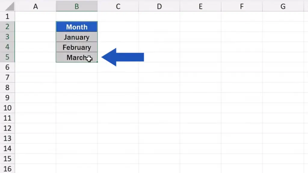
In the first step to transpose data in Excel, we need to select the relevant area we want to switch. We’ll work with the data stored here, in column B, so we’ll click on this column.

How to Copy and Paste Data for Transposing

Then, we press the right mouse button and choose the option ‘Copy’.

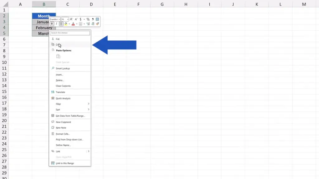
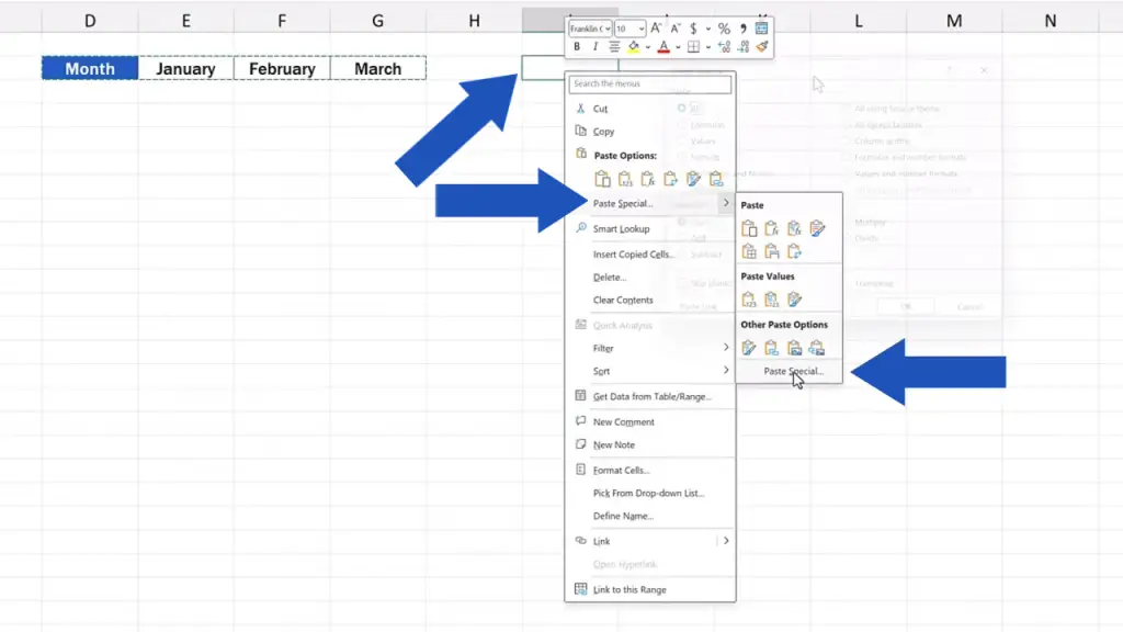
To carry on, we click on the cell where we want to store the first value – here we’ll click on D2. Now, we do a right click again, we choose ‘Paste Special’ and ‘Paste Special’ down here again.

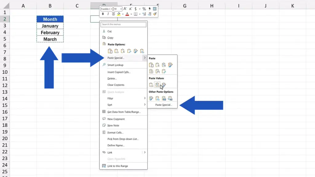
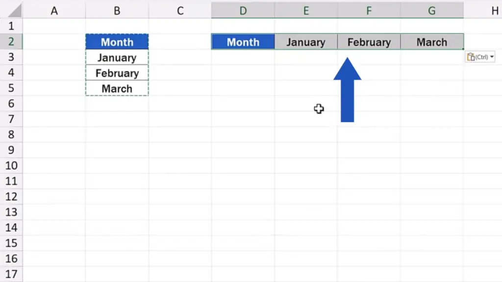
We can move the window a bit and down here we can find a useful feature ‘Transpose’. Thanks to this functionality, the data organised in the column will be switched and will show in a row. Let’s select the option, click on OK and here we go!

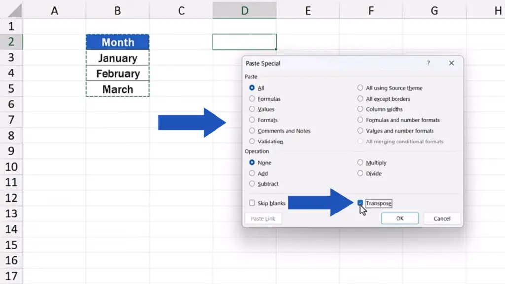
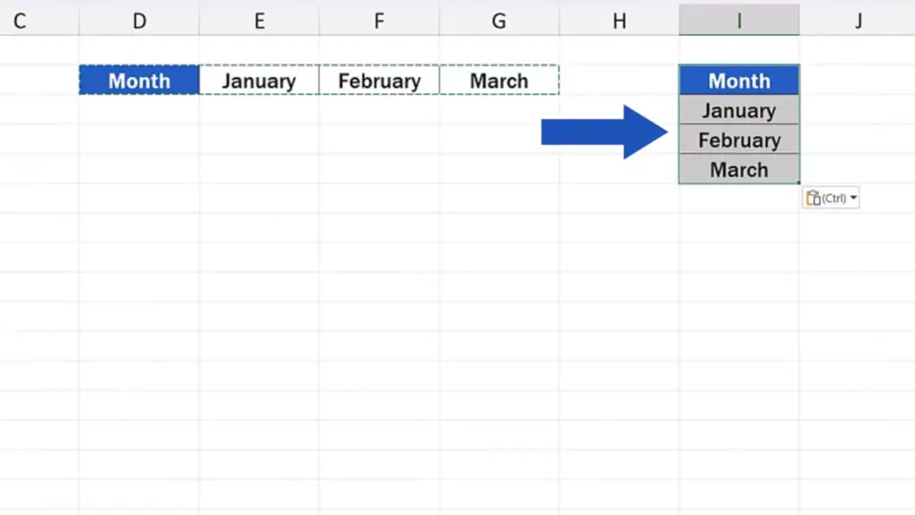
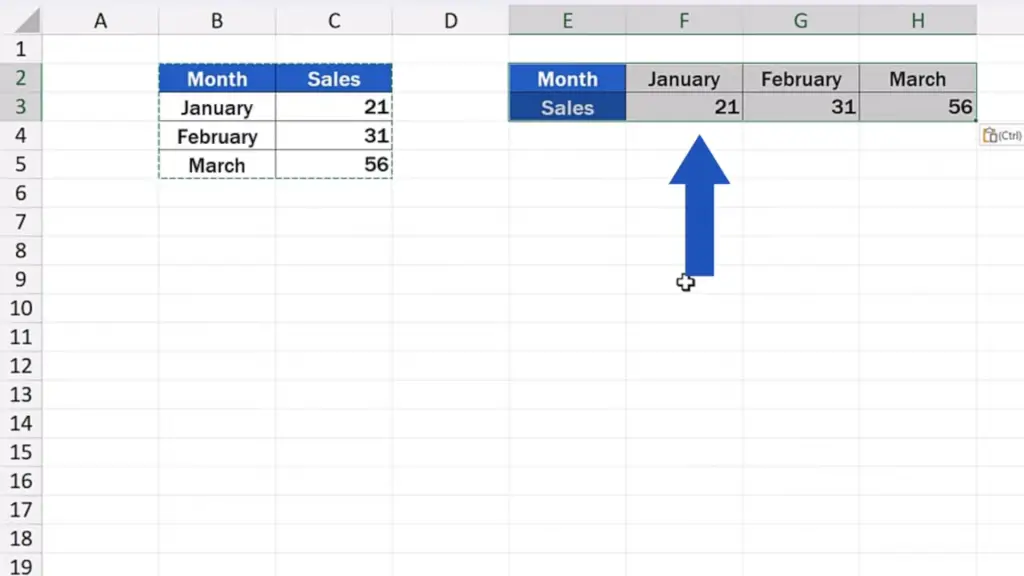
The data from column B now appear in a row.

How to Transpose Data from Rows to Columns

This also works when we want to arrange data the opposite way – from rows to columns. We just follow the same steps.

First, we select and copy the data.

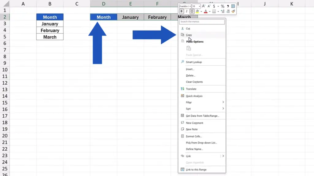
Then we click on the cell marking the target location for the data and now, through the option ‘Paste Special’, we use the feature ‘Transpose’ again.

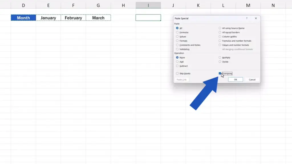
And here we go again! The data previously arranged in a row appear in a column.

How to Transpose Multiple Columns/Rows

And let’s move on. We can click into Sheet 2.

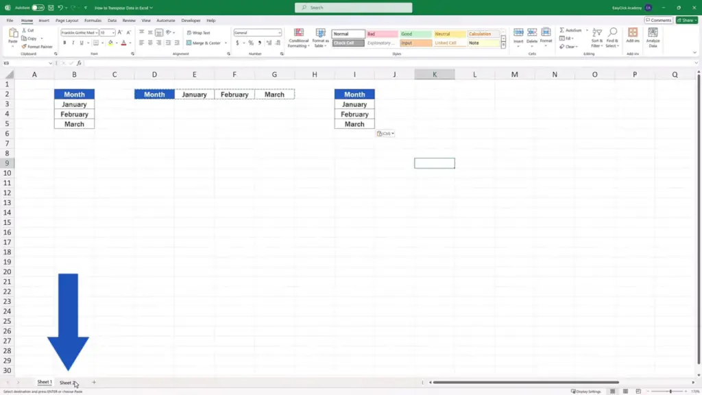
And have a look at how we can easily use the very same steps to transpose a number of columns or rows. To learn something new, we’ll use a shortcut key now.

Even when working with multiple columns, first, we need to select the relevant data range. The data can now be copied through the keys Control and C. Then we click on the cell which should become the top left corner of the transposed data area.

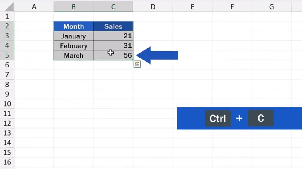
We click on E2 and here comes the time to use the hotkeys for opening the Paste Special window. Let’spress and hold the Alt key, then press E followed by S.

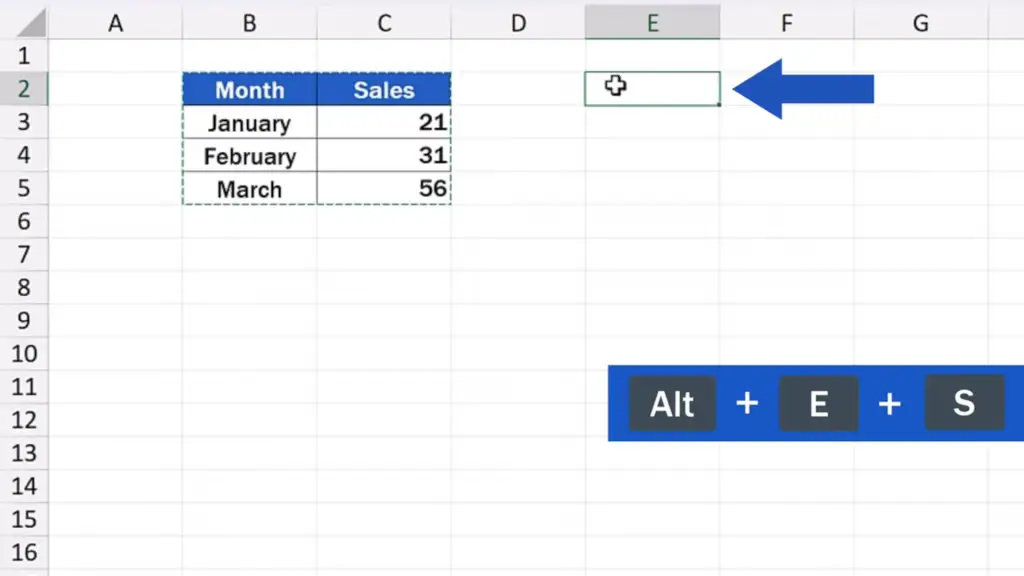
The window for Paste Special appears, we tick ‘Transpose’, press OK and that’s all it takes!

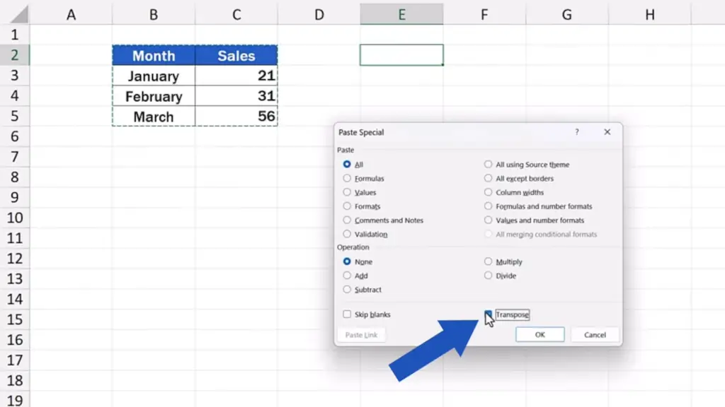
Data organized in multiple columns have been rearranged into rows. And you can follow the same steps if you want to switch rows into columns.

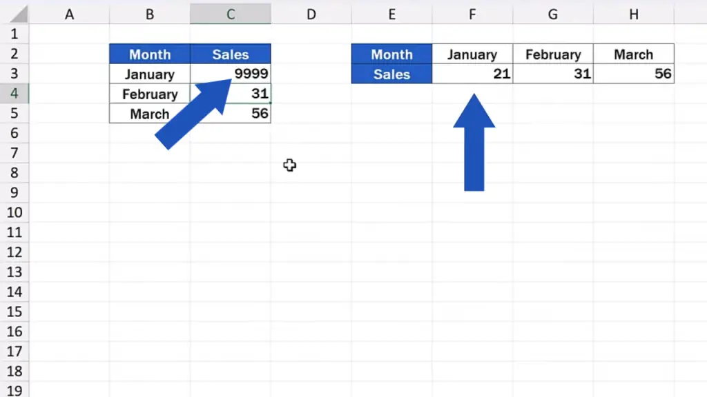
Before we wrap it up today, it’s important to note that such transposition is static, which means that if we change a value in the original data table, for instance in the cell C3, the transposed data in the switched cell F3 won’t change.

If you’d like to know how to make the transposition dynamic, do let us know! Leave a comment in the comments section below and we’ll be happy to share the trick with you in a separate video tutorial!

Don’t miss out a great opportunity to learn:

If you found this tutorial helpful, give us a like and watch other tutorials by EasyClick Academy. Learn how to use Excel in a quick and easy way!

Is this your first time on EasyClick? We’ll be more than happy to welcome you in our online community. Hit that Subscribe button and join the EasyClickers!

Thanks for watching and I’ll see you in the next tutorial!