How to Switch Rows and Columns in Excel (the Easy Way)

If you’d like to see the easiest way how to switch rows and columns in Excel, you’re in the right place!

Just keep reading!

See the video tutorial and transcription below:

See this video on YouTube:
https://www.youtube.com/watch?v=e4uwEtjjDII

How to Switch Rows and Columns in Excel – Paste Special Option

To switch rows and columns in Excel, select the area you want to switch in the first place. Right-click on the selected part and click on ‘Copy’.

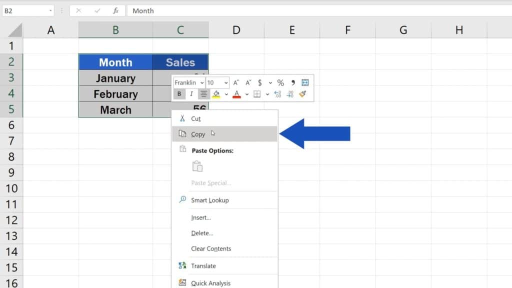
After that, click on the cell where you want to place the upper left-hand corner of the area that will contain the switched rows and columns.

Here, for example, we can click on the cell E2. Do a right-click and select ‘Paste Special’ and then ‘Paste Special’ again.

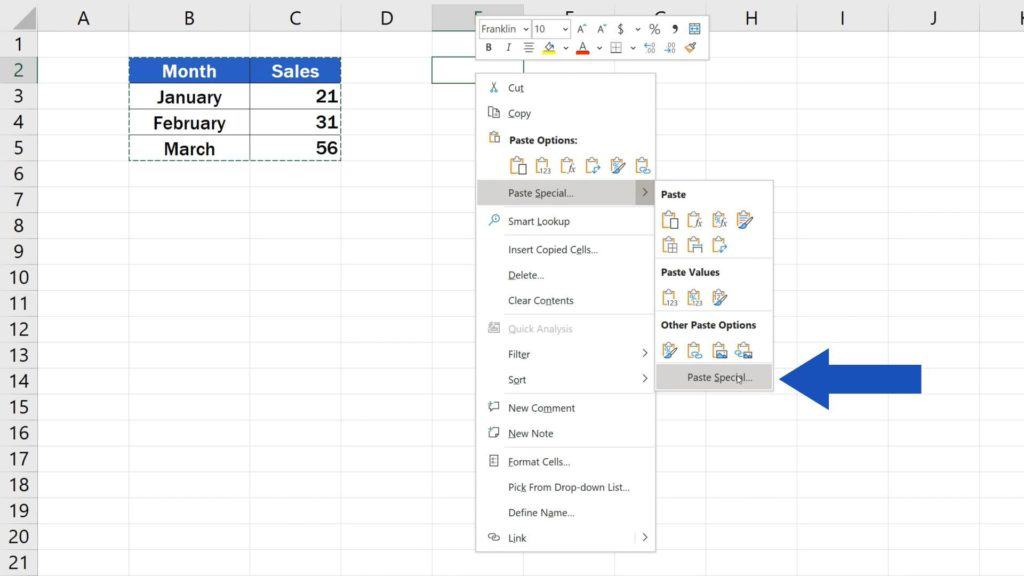
How to Switch Rows and Columns in Excel – ‘Transpose’ function

Right there you’ll find the function ‘Transpose’ which can switch rows and columns of a table.

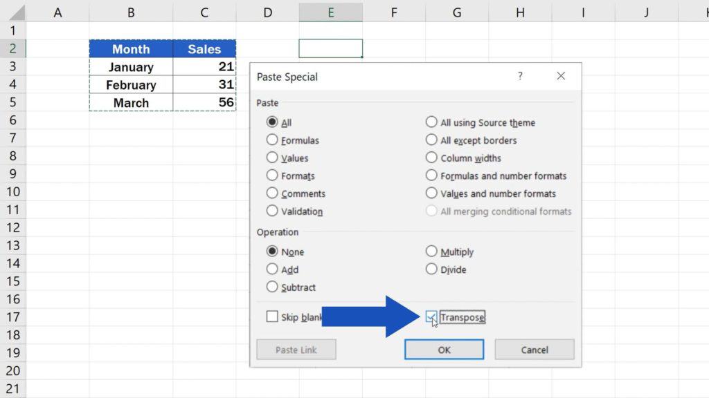
Select this function, hit OK and that’s it! A copy of the original data table has been created with its rows and columns switched.

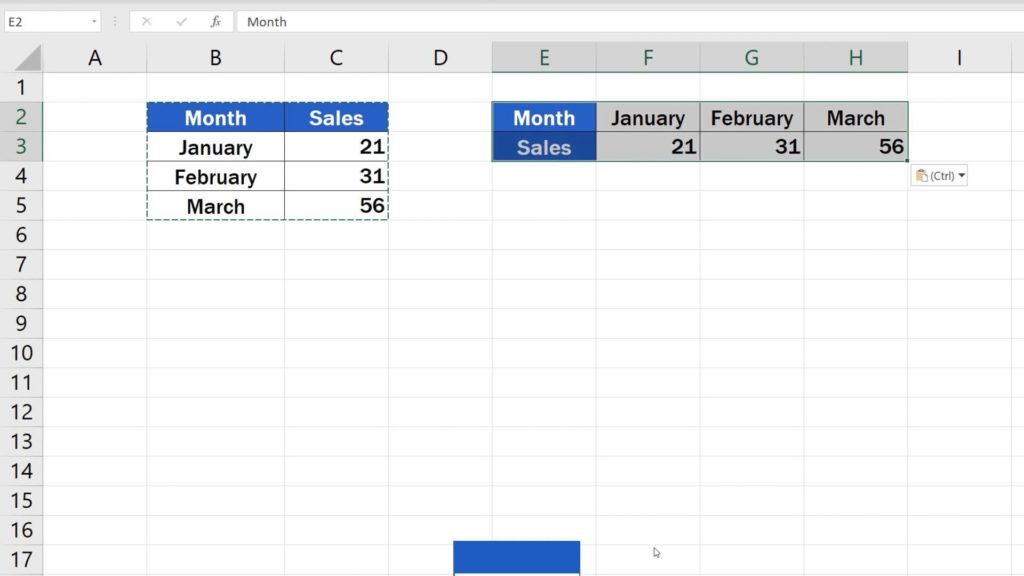
Remember, though, that this ‘Transpose’ function is static, which means that if you decide to change a value in the source table, for instance in the cell C3, the value in the switched table, in this case the cell F3, will stay unchanged.

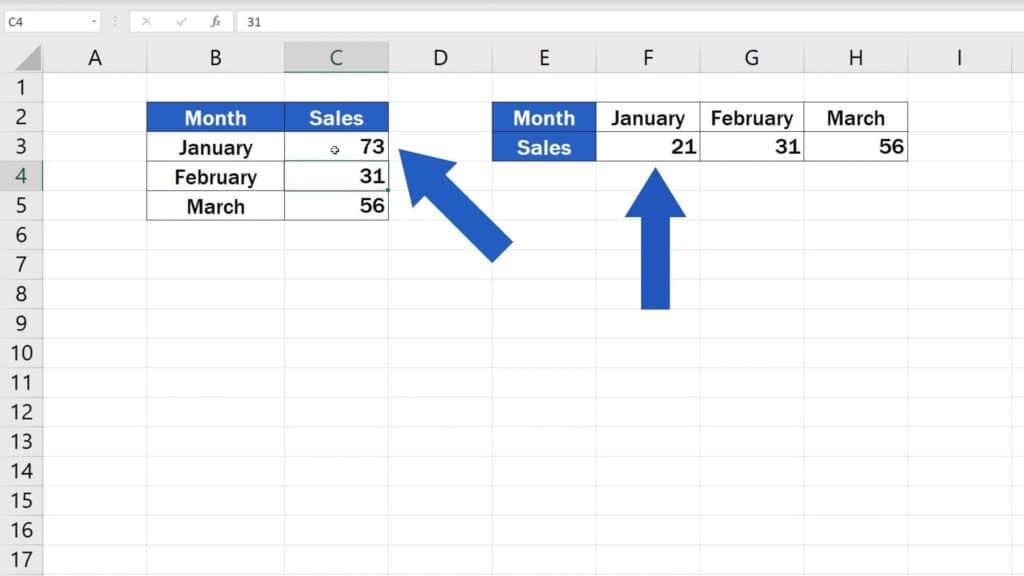
And here comes a question for you – is the static way of transposing data what you’re looking for or would you like to know more and learn how to switch rows and columns dynamically?

Make sure you’ll let us know in the comment section below – the EasyClick Academy team will be happy to help.

Don’t miss out a great opportunity to learn:

• How to Highlight Blank Cells in Excel (Conditional Formatting)
• How to Insert Symbol in Excel
• How to Use Color Scales in Excel (Conditional Formatting)

If you found this tutorial helpful, give us a like and watch other video tutorials by EasyClick Academy. Learn how to use Excel in a quick and easy way!

Is this your first time on EasyClick? We’ll be more than happy to welcome you in our online community. Hit that Subscribe button and join the EasyClickers!

Thanks for watching and I’ll see you in the next tutorial!