How to Sort Alphabetically in Excel

If you’re wondering how to sort data alphabetically in Excel, you’re in the right place! We’ll be talking about a function which you can use to sort a list of employees’ names, products, or any other list you need.

Ready to start?

See the video tutorial and transcription below:

See this video on YouTube:
https://www.youtube.com/watch?v=YNxvE6Fk630

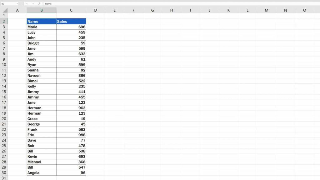
Sorting data alphabetically, whether A to Z or vice versa, Z to A, can be comfortably done in a table of any size. We’ll have a look at how to do it using this prepared table.

Two Types of Difficulties to Solve Before You Start

Before we start, let’s just discuss two types of difficulties you can encounter while sorting.

To avoid the first one, make sure that there are no blank entries or rows in the list before using the sorting function. Blank entries can easily happen if you’ve imported data from other applications. Now, imagine that we delete the data in row 10.

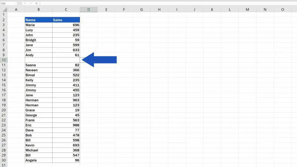
In that case, Excel would work only with rows 2 to 9 and data stored below the row 10 would get ignored and wouldn’t get sorted alphabetically.

Therefore, if a table you’re working with contains any blank entries, delete these rows and only then carry on with sorting. If the table you’re working with is extremely large, use the little trick we shared in the video tutorial on how to remove blank rows in Excel.

We’ll undo the last step to make sure all rows in the table are filled with data, and we’ll move on.

The second problem you may encounter is tied to the table headers.

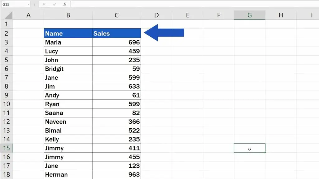
If you include headers in a table you prepared, it’s important that you distinguish it from the rest of the data. Because if you don’t, Excel will include the text of the header in the sorting as one of the list items, and that’s not what we want. It might be a good idea to use different colours or formatting to make the header of the table distinct and prevent this kind of issue.

Now, let’s assume you’ve done what was needed – the header has been formatted in a way that’s different from the rest of the data, and there are no blank entries in the table. We can move on to sort the data alphabetically.

It’s very simple and easy.

Sorting the Data Alphabetically A to Z

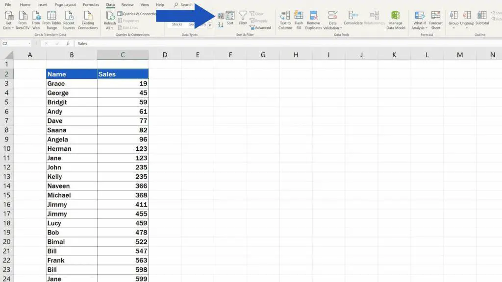
First, click on the header of the column which contains the list of data you want to sort. We’ll click on cell B2, because we need to sort the names of employees. Then we’ll click on ‘Data’ tab, section ‘Sort & Filter’ for two quick options to sort data – A to Z or the other way round, Z to A.

Here we’ll go for the first one – A to Z. Done!

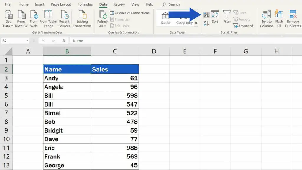
The names of employees have been sorted alphabetically, A to Z, just as we wanted. You can use the very same function to easily sort also numbers.

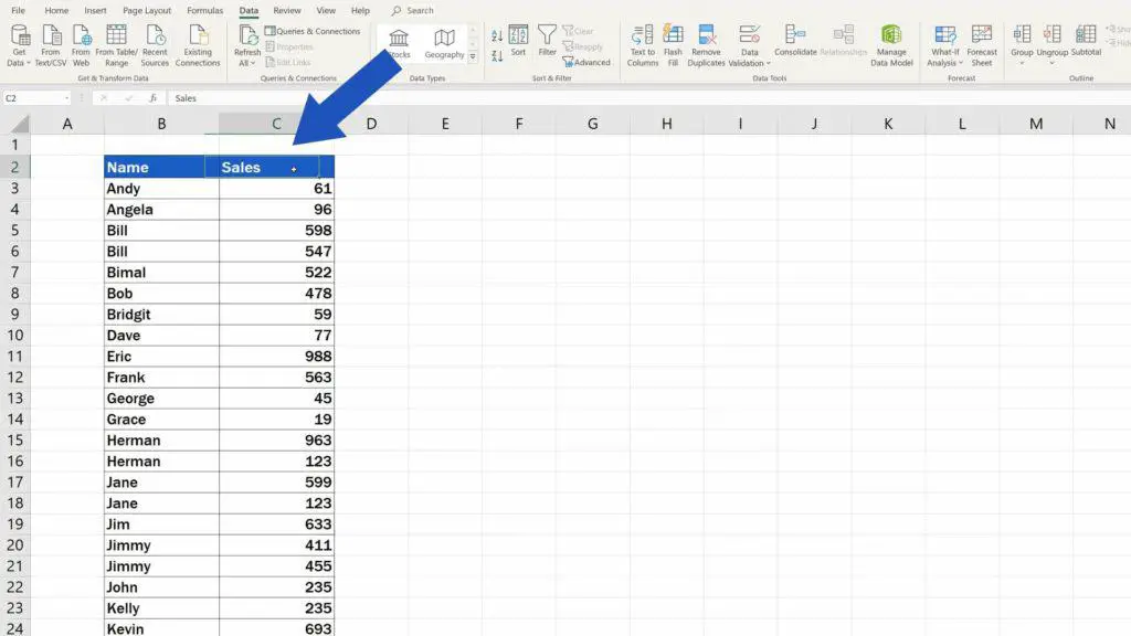
From lowest to highest or vice versa.

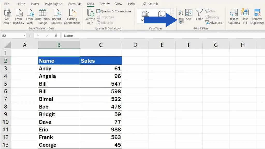
Sorting the Data Alphabetically Z to A

But now if we want to swap and sort the names Z to A, we can simply click on the button ‘Sort Z to A’ and the list gets sorted the way we need.

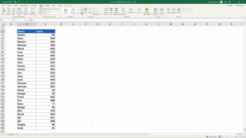
This function works with any number of data entries in tables of any size.

If you’re interested in learning more about a simple way of how to filter data, watch our upcoming videos by EasyClick Academy team!

• How to Create Filter in Excel
• How to Clear or Remove Filter in Excel
• How to Find the Largest Number in Excel
• How to Remove Blank Rows in Excel – ADVANCED

If you found this tutorial helpful, give us a like and watch other video tutorials by EasyClick Academy. Learn how to use Excel in a quick and easy way!

Is this your first time on EasyClick? We’ll be more than happy to welcome you in our online community. Hit that Subscribe button and join the EasyClickers!

Thanks for watching and I’ll see you in the next tutorial!