How to Show or Hide the Ribbon in Excel (Quick and Easy)

Today we’ll have a look at how to show or hide the ribbon in Excel. And you’ll see – it’s no rocket science.

Let’s get started!

Would you rather watch this tutorial? Click the play button below!

What Is the Ribbon in Excel and Where to Find It

The Ribbon in Excel is the display you see at the top of the Excel window, through which you can access Excel commands and functions.

How to Show the Ribbon in Excel

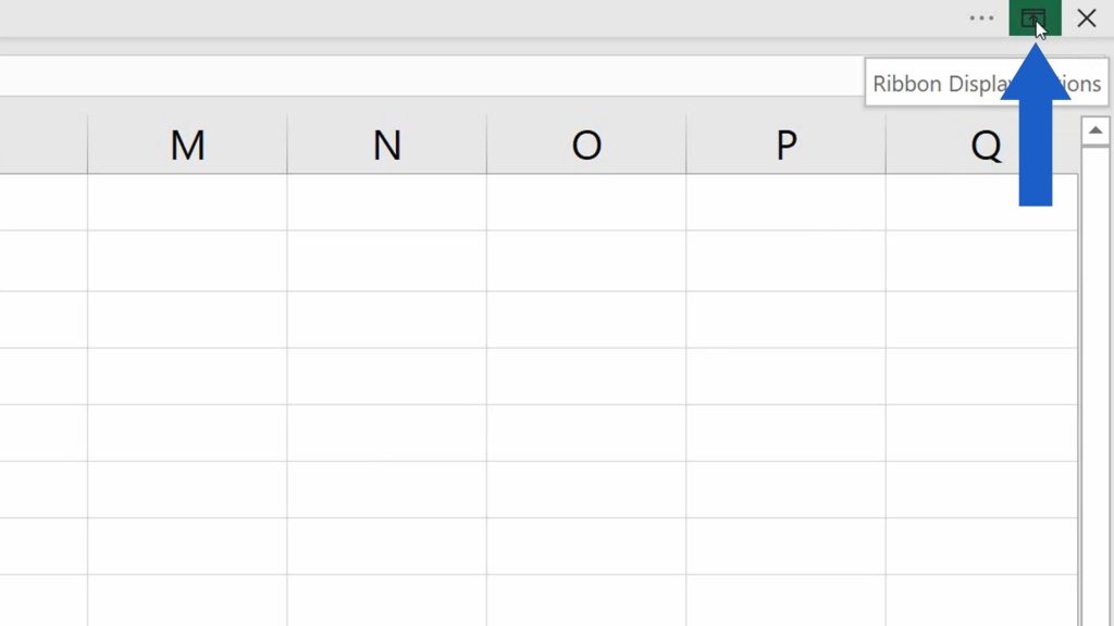
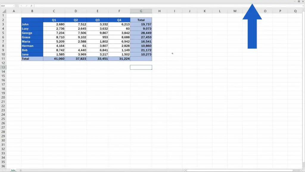
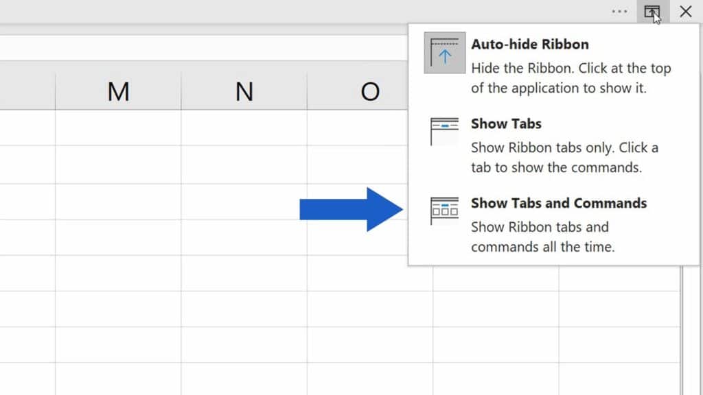
If it’s hidden and you want to see it, click on the icon in the top right-hand corner, the one with an arrow pointing up, which is the icon for Ribbon Display Options.

From the menu that appears, select ‘Show Tabs and Commands’.

Excel will immediately show the ribbon with all the functions Excel offers when the display is set on standard.

How to Hide the Ribbon in Excel

Now let’s have a look at the other two options how you can make your working area in the spreadsheet larger.

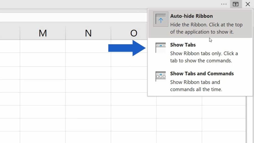
To see all Ribbon Display Options again, click on the arrow icon on the right at the top of the screen.

Let’s select the first option, ‘Auto-hide Ribbon’, and let’s see what happens now.

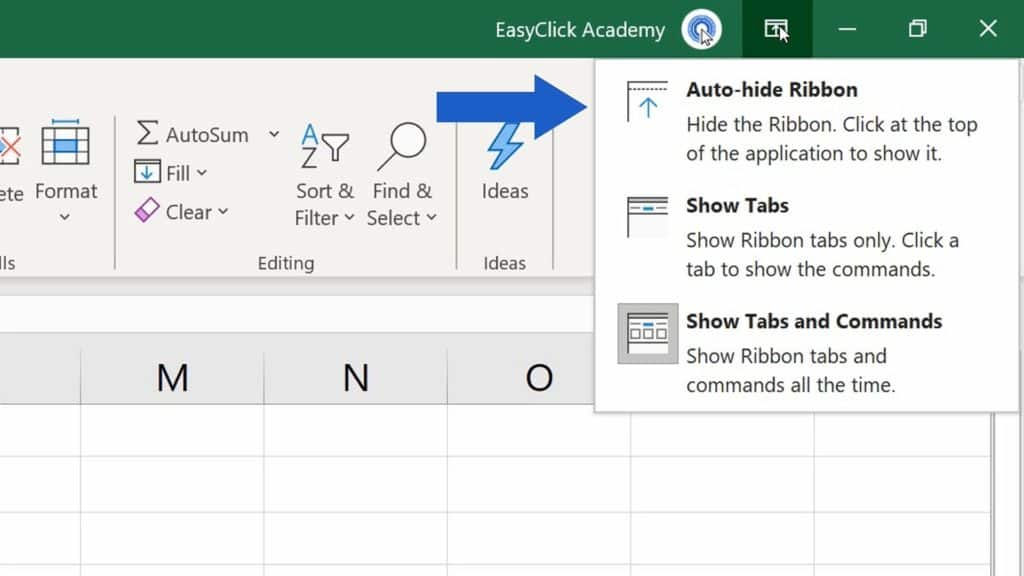
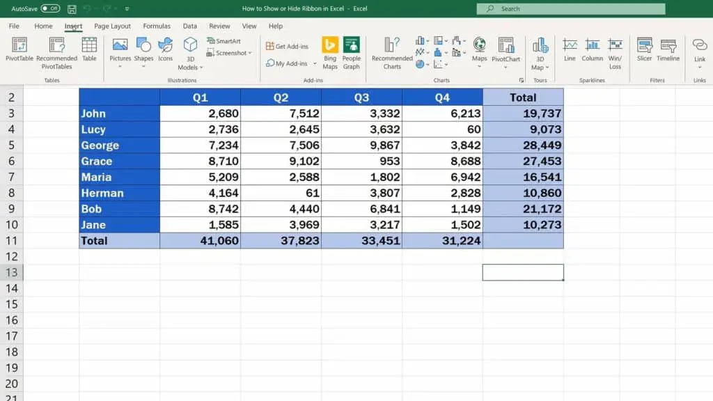
This option hides the ribbon, but once we need it, we can always ‘call’ it by clicking into the bar located at the top of the window.

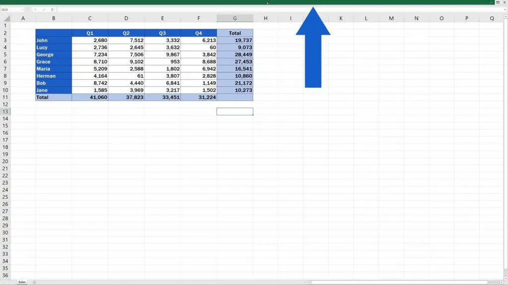
The ribbon will appear and you’ll be able to choose whichever function you need.

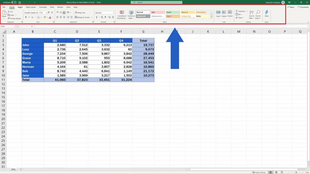
Then you click anywhere within the spreadsheet area and the ribbon will disappear again. Once it’s not visible, you can work with the spreadsheet extended full screen.

And there’s one option left to explore.

How to Show Ribbon Tabs Only

So, let’s click on the Ribbon Display Options icon again, but now select ‘Show Tabs’.

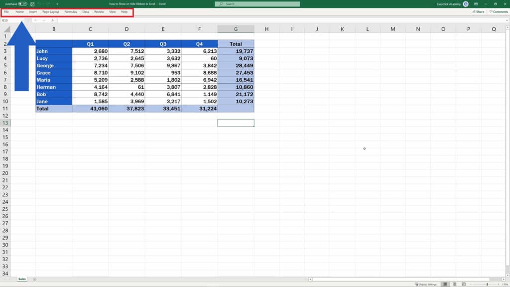
In this view, you’ll see individual tab names.

Whenever needed, just click on a tab name and you’ll see the options of the tab that were previously hidden.

Pick the function you need and click anywhere in the spreadsheet area to hide the options again. Only tab names will stay visible.

How to Switch between All Views

To switch views according to what you need is easy – simply click on the icon in the top right-hand corner and choose whichever view suits you best. To get back to the standard view, go for ‘Show Tabs and Commands’, where all the tab names and the options are visible at all times.

And if you want to extend the working area of the spreadsheet even more, there’s another little trick that will help you.

If you’re interested in learning how to show or hide the formula bar in Excel, watch the next EasyClick Academy tutorial! You can find the link in the list below.

Don’t miss out a great opportunity to learn:

• How to Show or Hide the Formula Bar in Excel (Quick and Easy)
• How to Move Columns in Excel (The Easiest Way)
• How to Move Rows in Excel (The Easiest Way)
• How to Delete Columns in Excel
• How to Create a Drop-Down List in Excel

If you found this tutorial helpful, give us a like and watch other video tutorials by EasyClick Academy. Learn how to use Excel in a quick and easy way!

Is this your first time on EasyClick? We’ll be more than happy to welcome you in our online community. Hit that Subscribe button and join the EasyClickers!

Thanks for watching and I’ll see you in the next tutorial!