How to Merge Two Columns in Excel (Quick and Easy)

This video tutorial offers a step-by-step guide on how to merge two columns in Excel. In our example, we’ll merge a person’s first name and surname in a separate column in a quick and easy way. The same way works if you’d like to merge larger amounts of data to avoid tedious typing and copy-pasting.

Contents hide

1 How to Use CONCATENATE to Merge Cells

2 How to Merge Multiple Columns in Excel

3 How to Add Spaces or Symbols Between Merged Data

4 How to Convert Merged Data to Values

How to Use CONCATENATE to Merge Cells

To merge two columns in Excel, first, we need to select a target cell. Here we’ll use the cell D3, so we click on it.

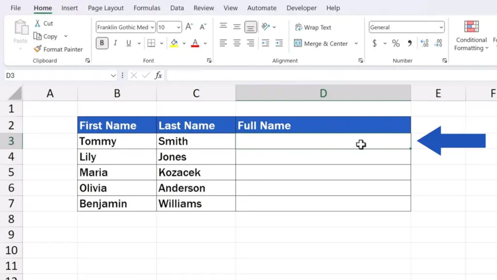
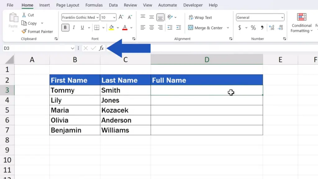
Then we click on the button marked with ‘f_x’ up here, which is the ‘Insert Function’ button.

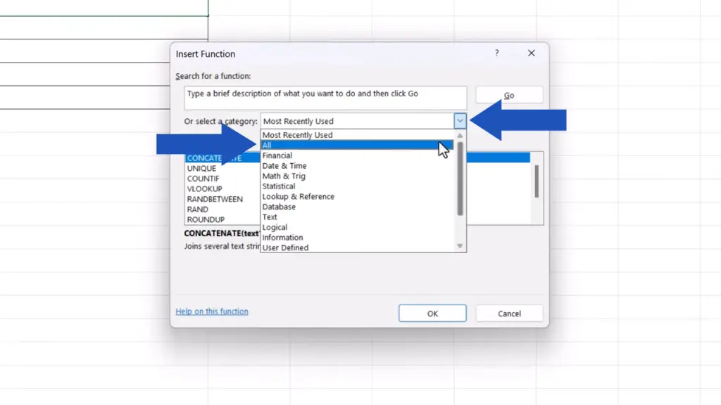
In the pop-up window that’s just appeared, we select the category ‘All’ and look for the function CONCATENATE.

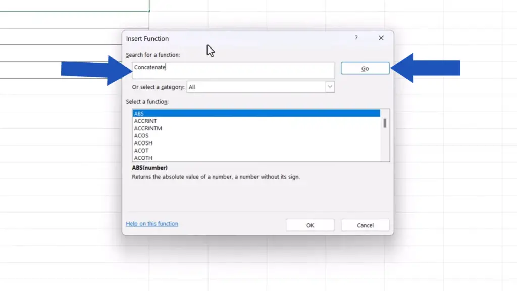
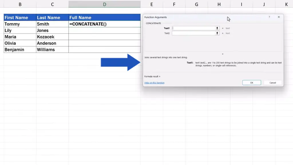
Now we click on OK, and here pops up another window where we can easily merge the data from these two columns.

How to Merge Multiple Columns in Excel

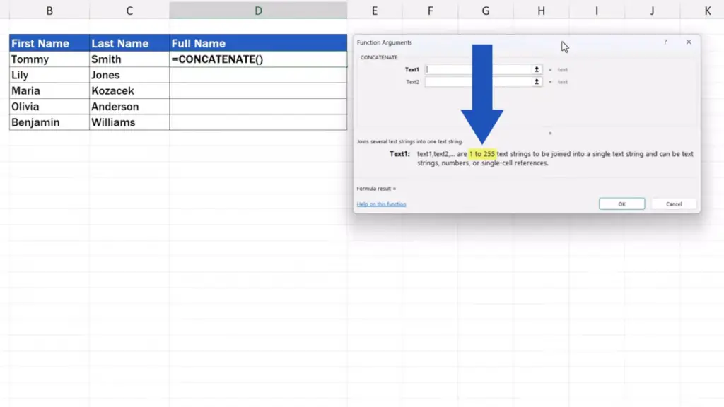
Thanks to the function CONCATENATE, you can merge up to 255 different items in one cell.

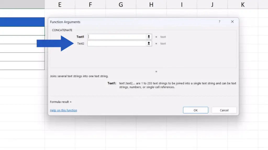
But first, you’ll see only these two fields – ‘Text1’ and ‘Text2’. Here you can enter the data to be merged.

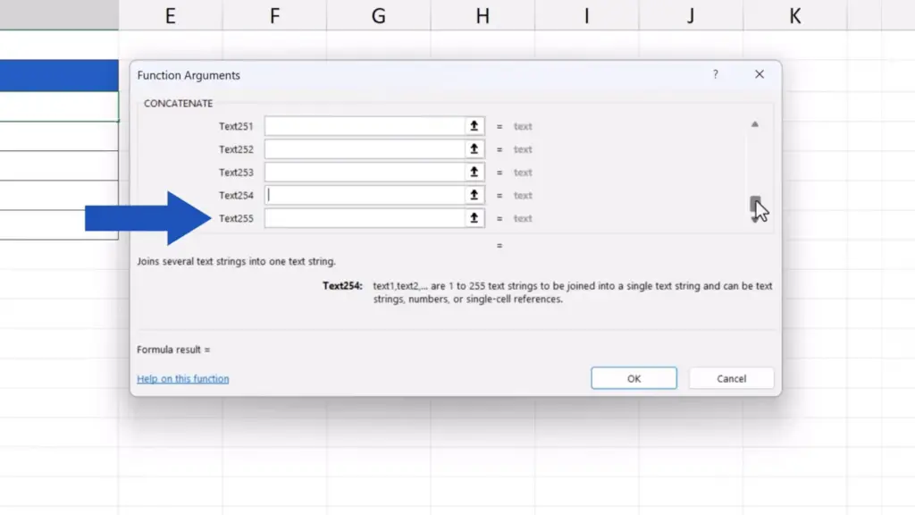
If you’d like to merge more items than just a first name and a surname, more fields will automatically appear once you click into the last visible box. This way, Excel can gradually open up to 255 text fields.

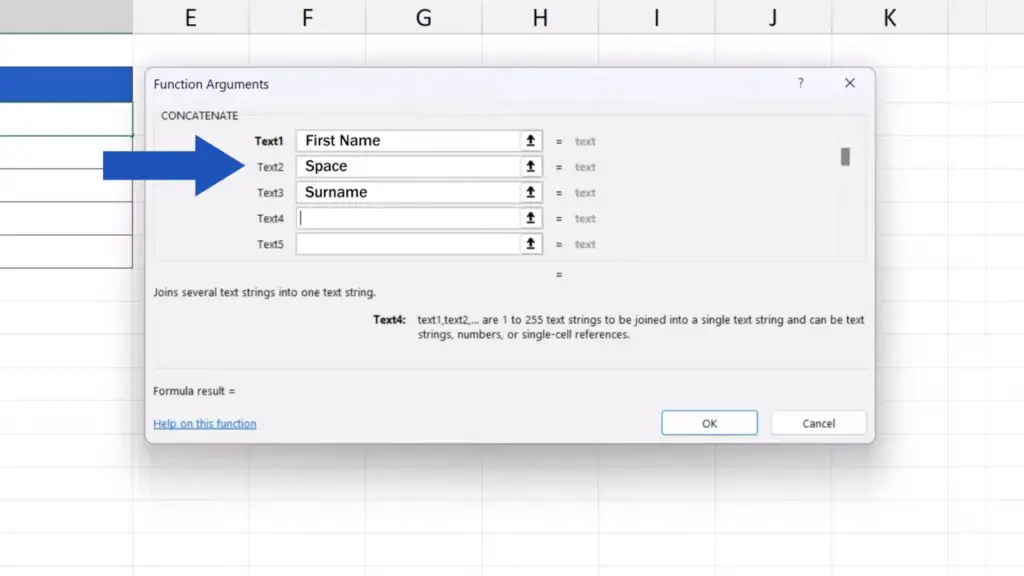
Let’s have a look at how we can enter data into the fields. We want to merge and create a full name in the format: first name – space – surname.

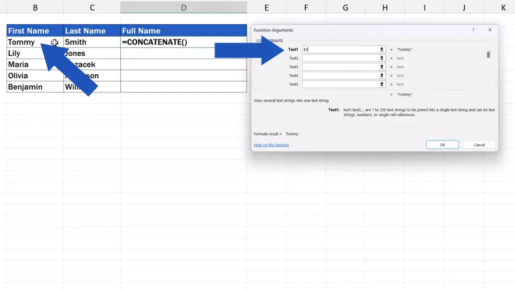
In ‘Text1’, we need to enter the first name. So, we click into the field ‘Text1’, then we click on the cell containing the value we want to use, in this case B3.

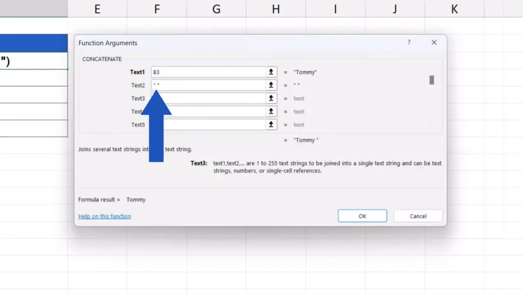
If we want to add a space between the first name and the surname, we need to enter a space in the field ‘Text2’, which is very easy – we just click into the box and press the spacebar.

As soon as we click into ‘Text3’, Excel will encode the space by adding quotation marks around it. The same way we can add for example a dash, a colon, or any symbol we need.

We’ll keep the space in ‘Text2’ and move on.

In ‘Text3’, we enter the surname again, by clicking into the box and then selecting the cell C3, which contains the data we need.

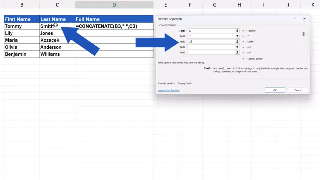
As we are joining the strings, here we can see a preview of the full text.

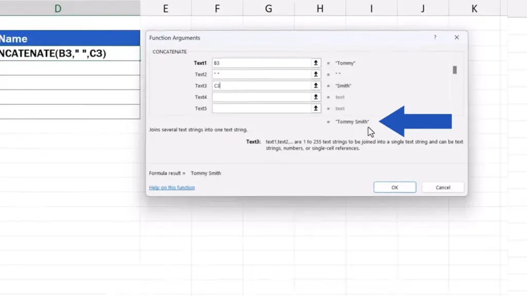
Once we’ve merged all the data, we click on OK and that’s all it takes!

How to Add Spaces or Symbols Between Merged Data

The first name and the surname have been joined without tedious typing or copy-pasting.

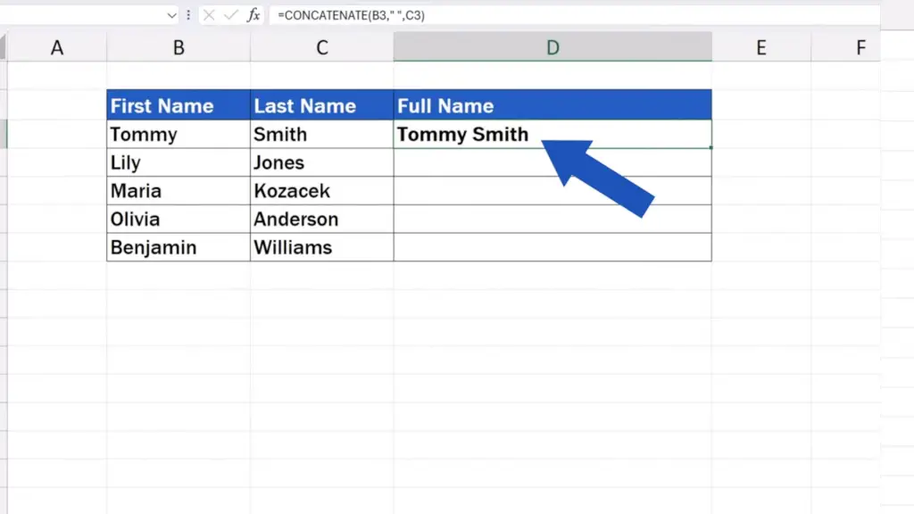
To merge the data in the rest of the rows, we don’t need to repeat these steps row by row.

We can just set the cursor on the cell containing the inserted function and drag its bottom right-hand corner down all the rows where we want the function to do the trick. Like this.

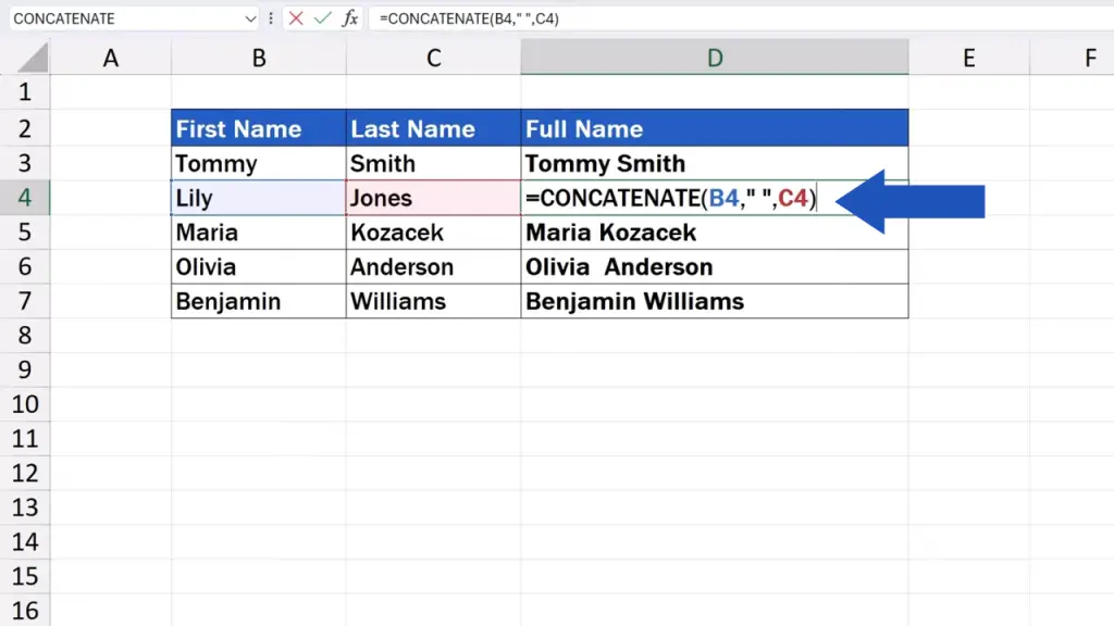
And before we wrap it up, there’s one important thing to remember.

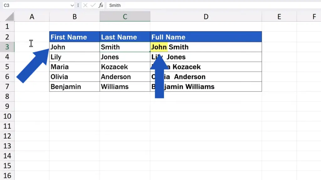
To change a merged text in a target cell, we need to change the information in the source cell first.

This is because the target cells do not contain the text itself but rather the function CONCATENATE which takes data from the columns we’ve merged.

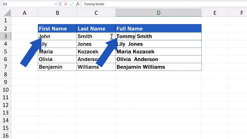
So, let’s say we’d like to change the name Tommy to John. To do that we need to navigate to cell B3 and make the change right there. The text in D3 will change based on what we’ve done in B3.

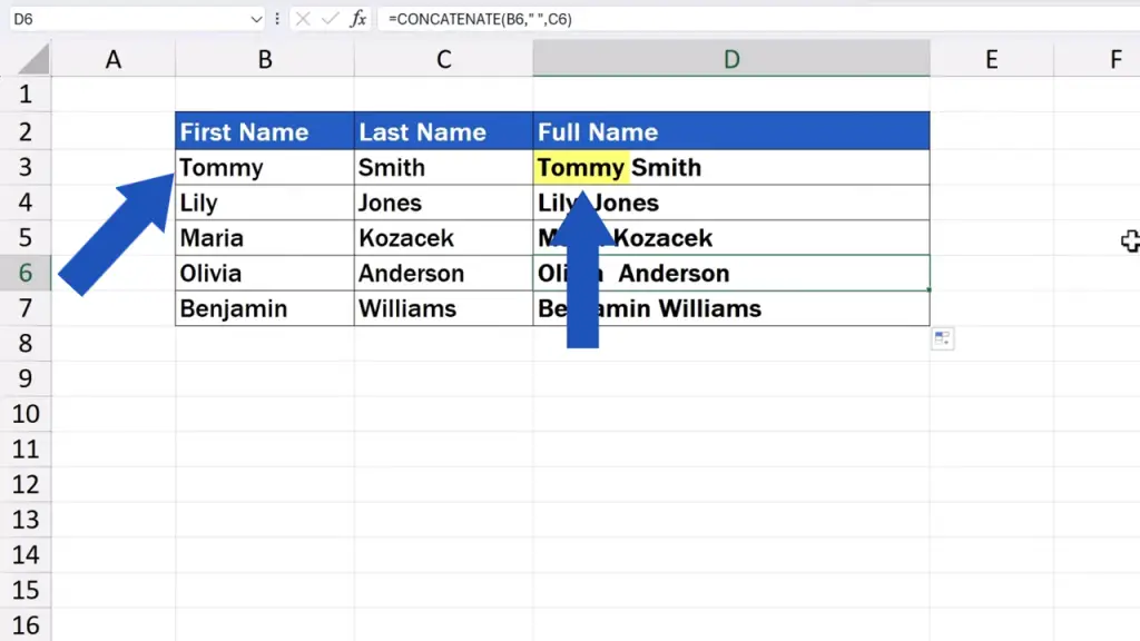
How to Convert Merged Data to Values

And if you’d like to keep just the text in the merged column rather than the function, it’s no rocket science either!

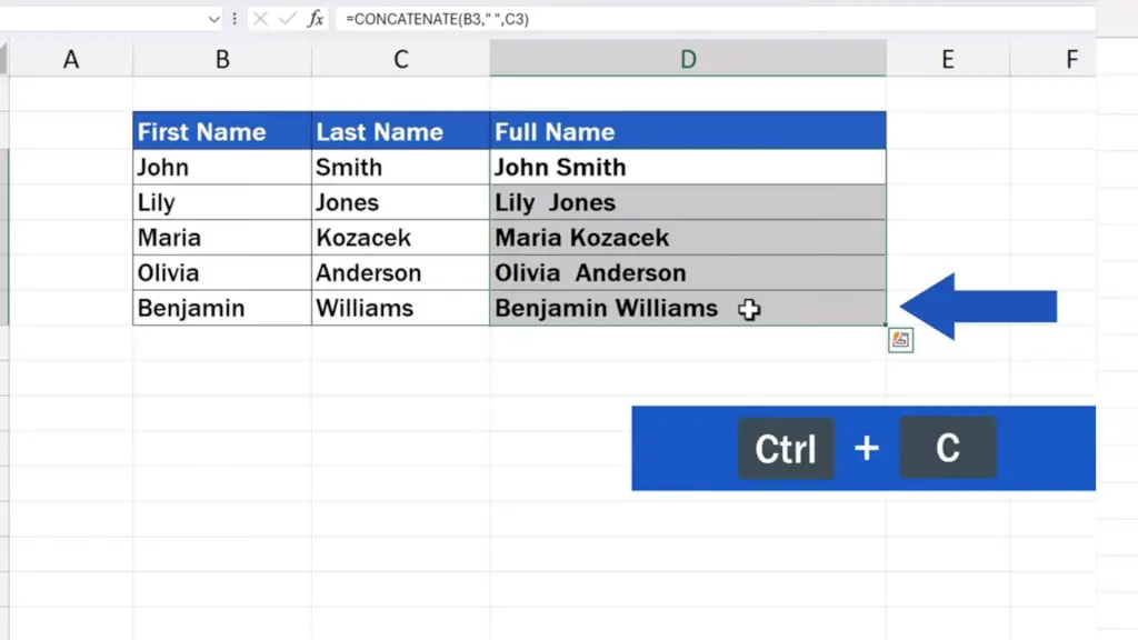
First, copy the data in the merged column using the Control key and C.

Then press the right mouse button and choose ‘Paste Special’ options. Here we’re going for the option ‘Values’.

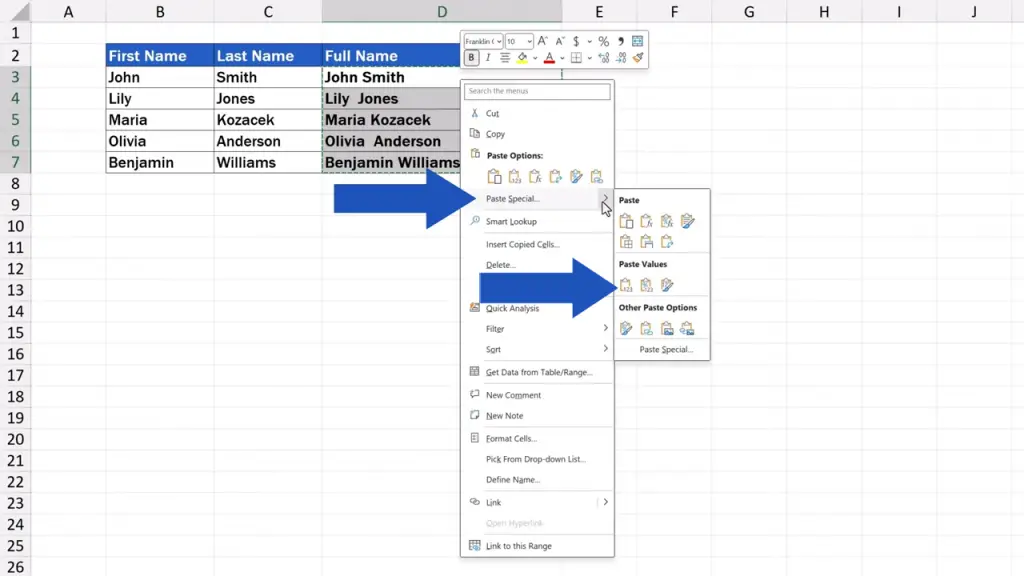
This will turn the function inserted in the merged column into the resulting values and you can further work with the text itself and modify it as you like.

Don’t miss out a great opportunity to learn:

How to Separate Names in Excel

If you found this tutorial helpful, give us a like and watch other tutorials by EasyClick Academy. Learn how to use Excel in a quick and easy way!

Is this your first time on EasyClick? We’ll be more than happy to welcome you in our online community. Hit that Subscribe button and join the EasyClickers!

Thanks for watching and I’ll see you in the next tutorial!