How to Merge Cells in Excel

In this tutorial you’ll see a quick guide on how to merge cells in Excel, which is a smart way how to format your data table!

Let’s see how to do it!

See the video tutorial and transcription below: 

See this video on YouTube:  
https://www.youtube.com/watch?v=hRlrj_np0Tw

Merging cells in a spreadsheet means that either a larger or a smaller group of separate cells will be joined into a single large cell that will take the whole area of the group.

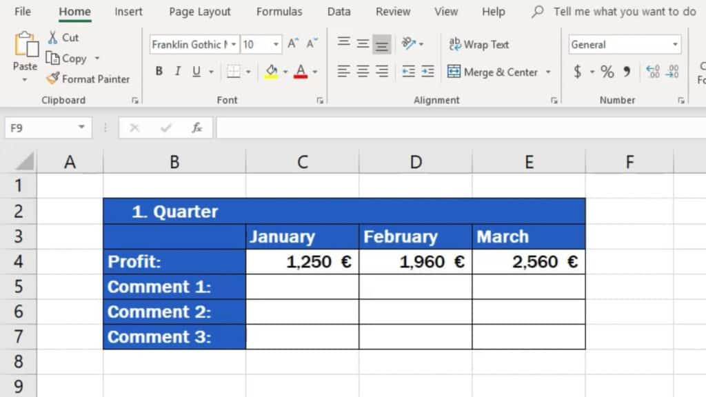
There are several ways how to do this in Excel, but we’re gonna have a look at one only – the most effective and efficient way.

Go to ‘Home’ tab, specifically the ‘Alignment’ section, and find the four options available there. These options offer four ways how you can merge but also unmerge cells. I will now explain each option on a specific example.

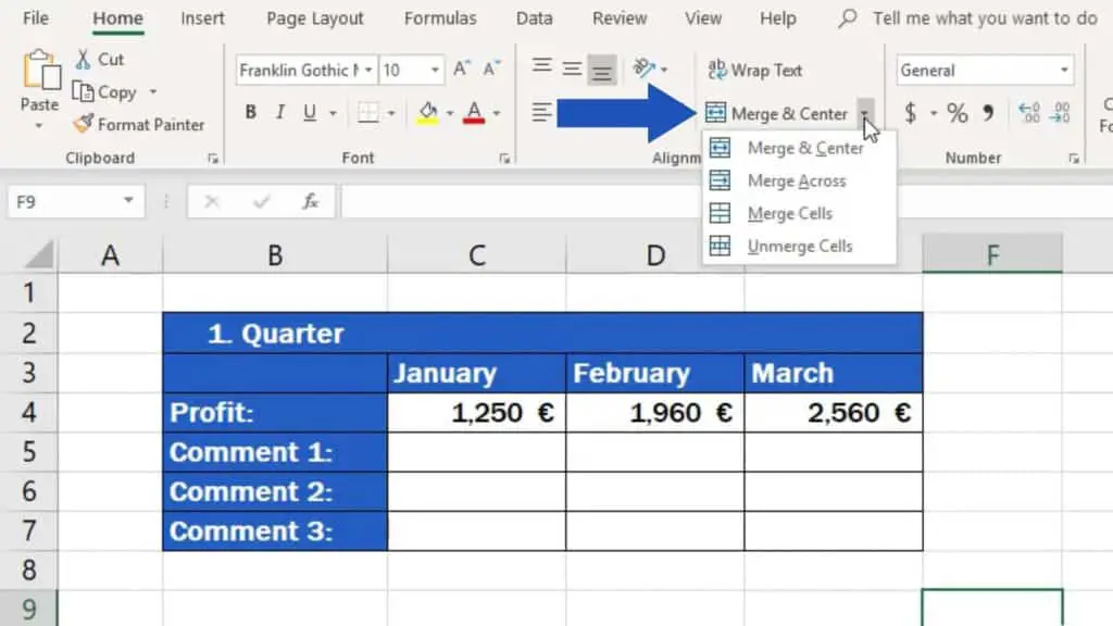
First, select the cells you want to merge. If the header of the table should be positioned right in the middle, use the first option ‘Merge & Center’. But if you don’t want to centre the text in the header, go for the third item from the top – ‘Merge Cells’. We now want the text to appear in the middle, so we’ll select ‘Merge & Center’.

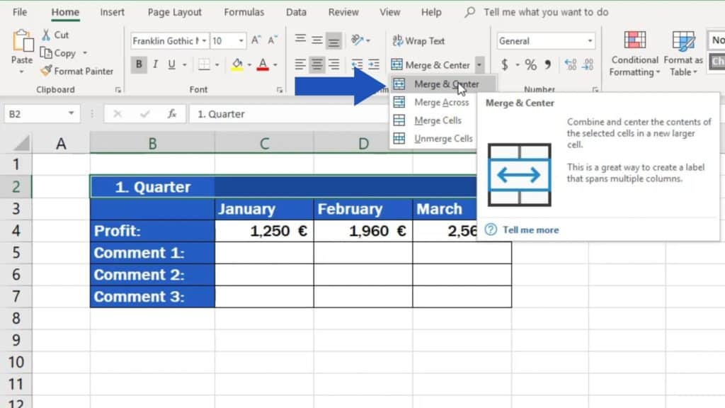
All four cells will be joined into one and the text will appear in the middle.

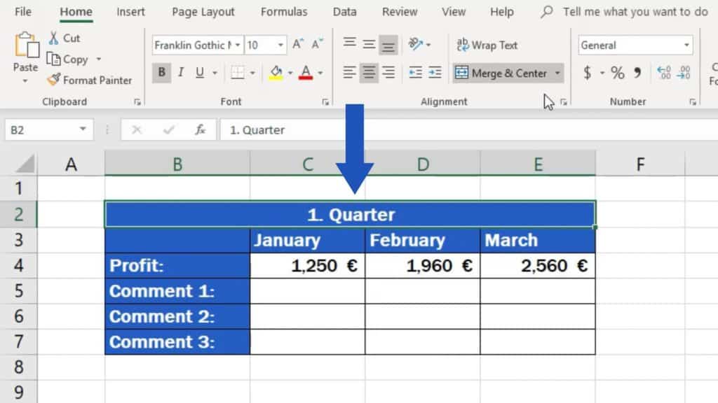
Let’s move on now!

How to Merge Cells Horizontally in Excel

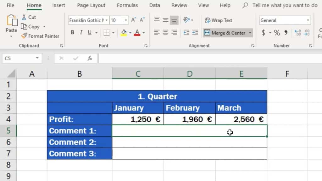
If you want to merge cells horizontally, to make rows, select the area in which you want to apply the formatting and click on ‘Merge Across’.

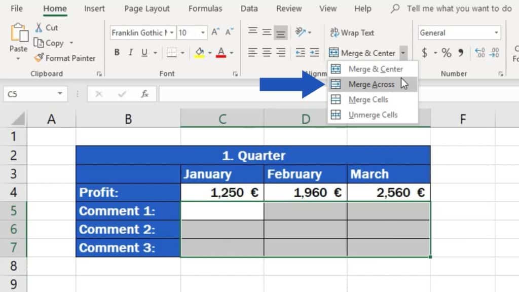
This will create some space for notes and comments.

How to Unmerge Cells in Excel

When formatting the table, you might also need to undo the merging at some point, to get the cells back into their original state. Trust me, it’s a piece of cake! Select the whole area you want to unmerge and click on the last option ‘Unmerge Cells’.

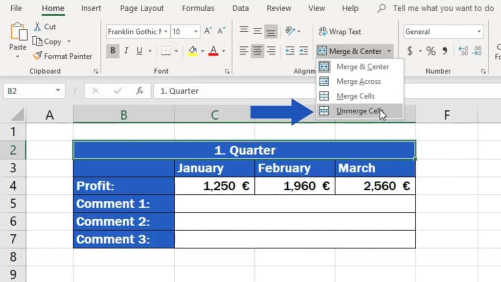
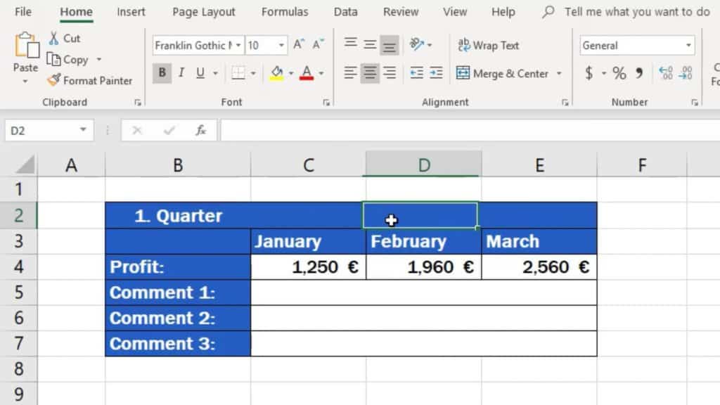
And that’s done! Each cell is now separate again.

Useful Excel Tip

And before we finish, here’s a useful tip – it’s always better to merge cells containing no text at all or with text in one cell only. If we wanted to merge let’s say these cells, each containing information about months, Excel will display a warning message that the cells will be merged, but only data in the cell in the top left corner will show in the merged area.

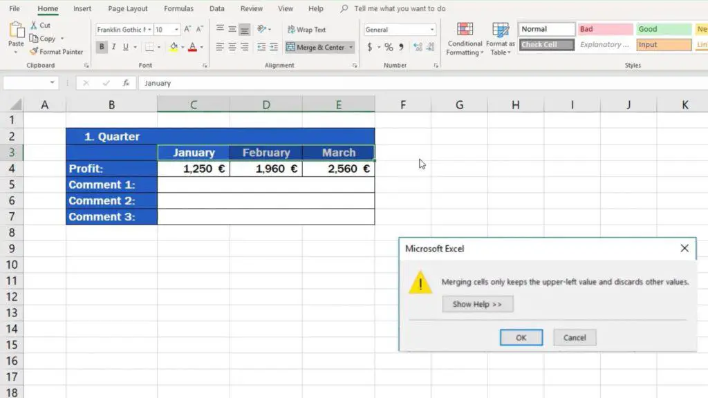
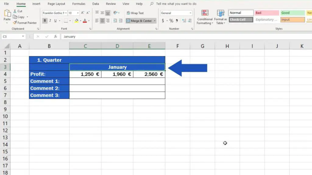
The contents of the rest of the cells will be deleted. So here we would be left only with ‘January’ and the information of the other two months would be removed.

Would you like to know:

• How to Change Text Direction in Excel
• How to Wrap Text in Excel
• How to Insert and Format Time in Excel

If you’ve found this tutorial helpful, like us and subscribe to receive more videos from EasyClick Academy. Look at more tutorials that help you use Excel quick and easy!

See you in the next tutorial!