How to Make Borders in Excel

Today’s tutorial is about how to make borders in Excel. And not only that! We’re gonna have a look at how to erase or remove the borders completely.

Let’s start!

Would you rather watch this tutorial? Click the play button below!

How to Make Borders in Excel

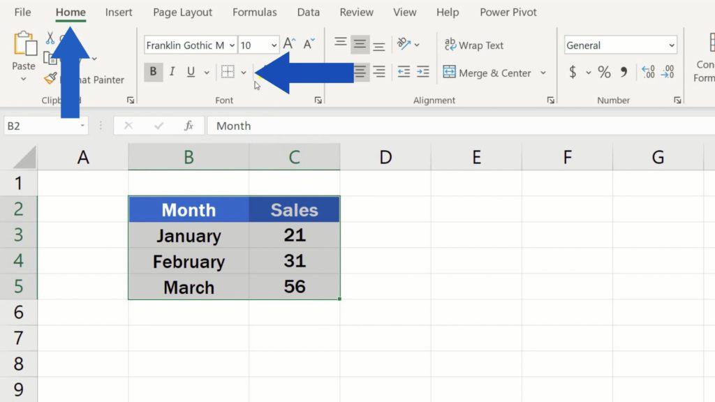
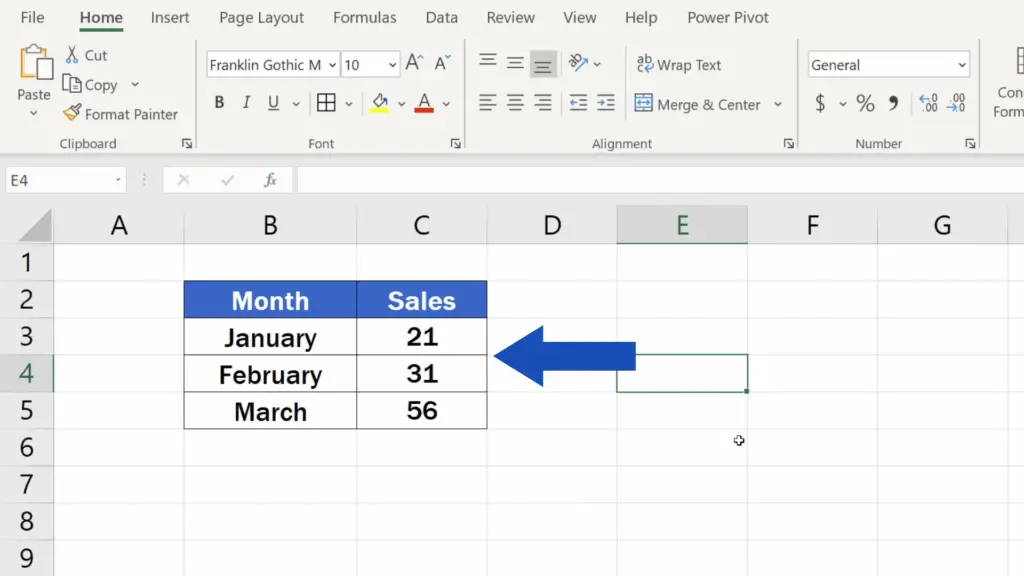
To draw borders in Excel, we need to select a relevant table area first.

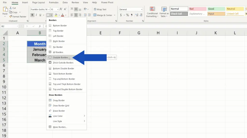
Then we go to the Home tab, click on this little arrow next to the icon for ‘Borders’ and choose the bordering we want to apply.

We’ll select ‘Outside Borders’ and Excel immediately makes a border around the table.

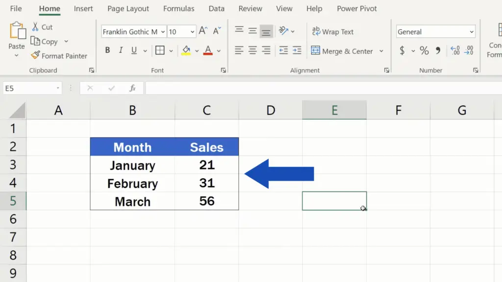
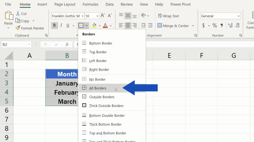
To draw borders around each cell within the table, select the area again and now choose the option ‘All Borders’.

How to Adjust the Borders

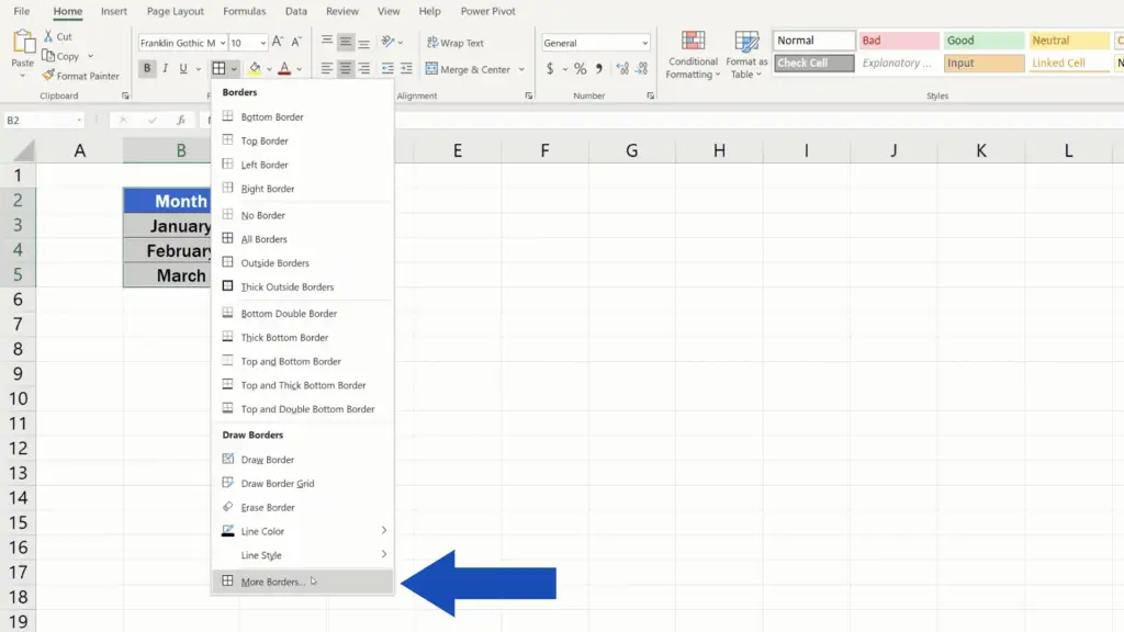
If you’re looking for something different, you can use any style of borders you want. Simply, click here on ‘More Borders’ and under the tab Border you’ll find everything necessary to adjust the borders according to what you need.

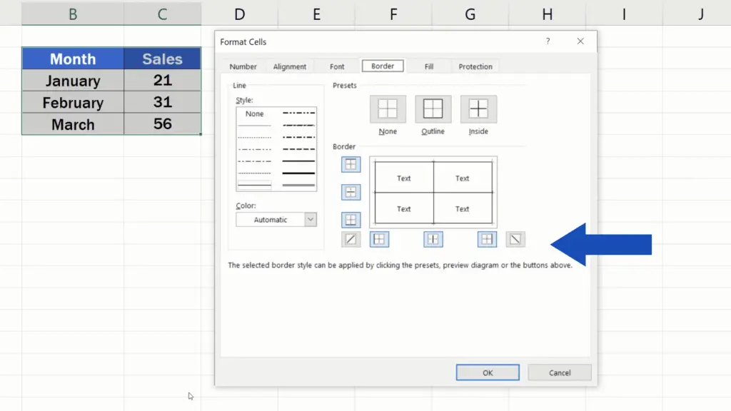
So, let’s say we want to use a double line for the outside border. Look for the double line in the section ‘Style’, select this type of the line.

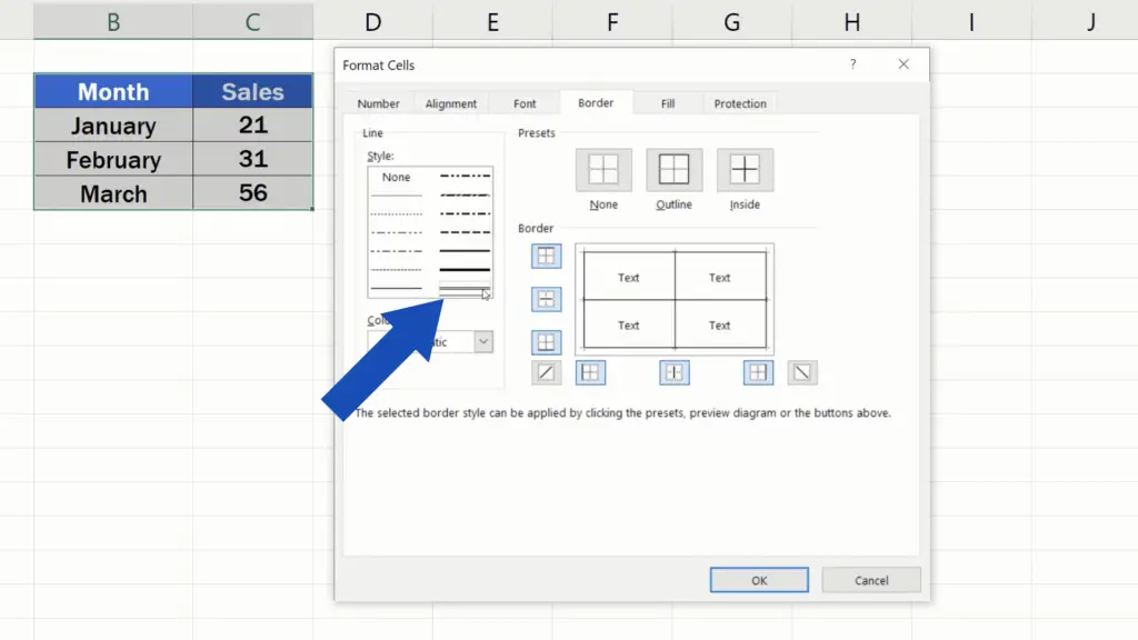
And now we need to define where we want to use the double line, so we’ll click on ‘Outline’ right over here.

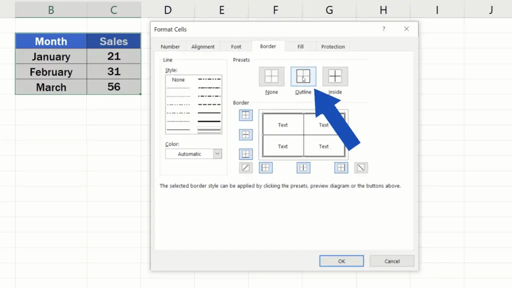
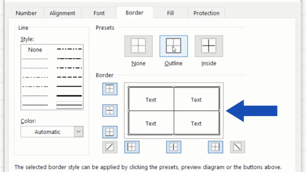
We can check the preview of what the borders will look like once applied here.

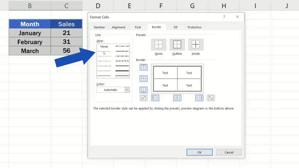
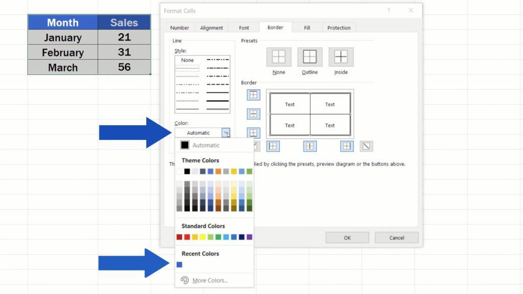
In a similar way, we can choose the colour of borders. For example, we want to use this dotted line style inside the table, so we’ll click on it, but we also want it to show in blue.

To do that, we need to go to the option ‘Color’ and select the shade of blue we want to use.

The button ‘Inside’ located here at the top of the window will apply these settings to the inside borders.

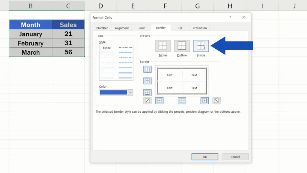
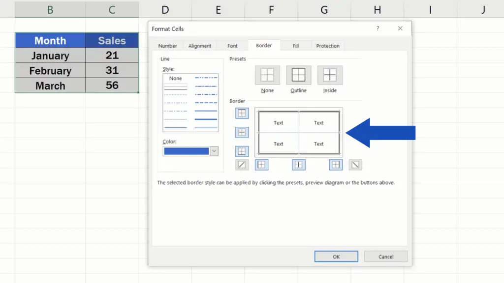
Have a look yourself and try out other possible options provided here, in this window!

As soon as everything’s been set, just click on OK to apply the changes and that’s it!

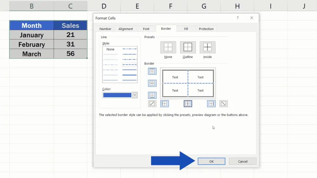
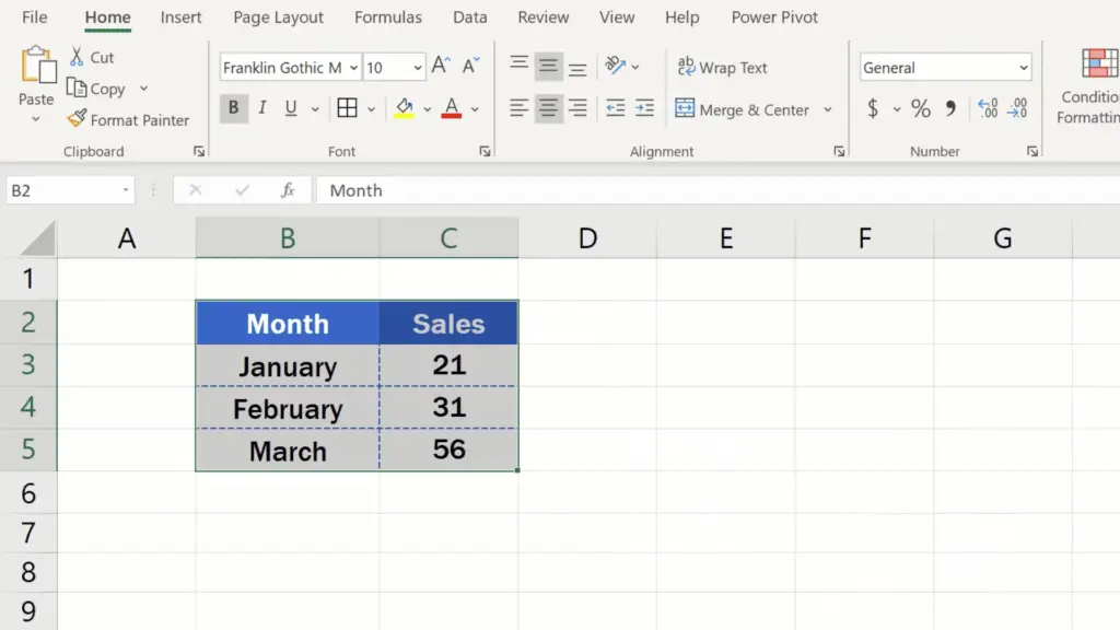
But before we wrap it up for today, let’s have a look at one more thing.

If you decide to remove the borders, there’s more than one way to do that.

How to Remove the Borders Only Partly

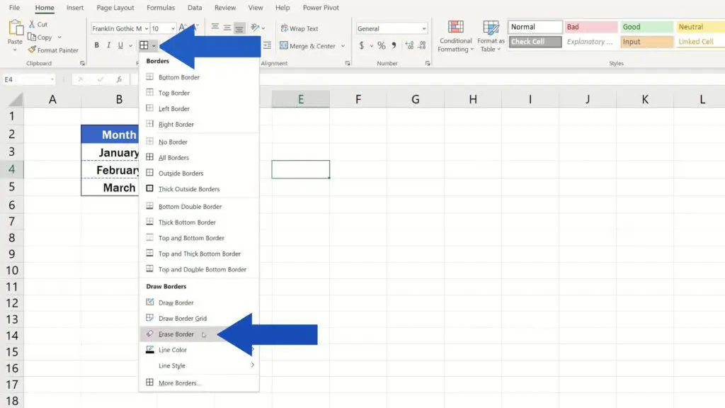
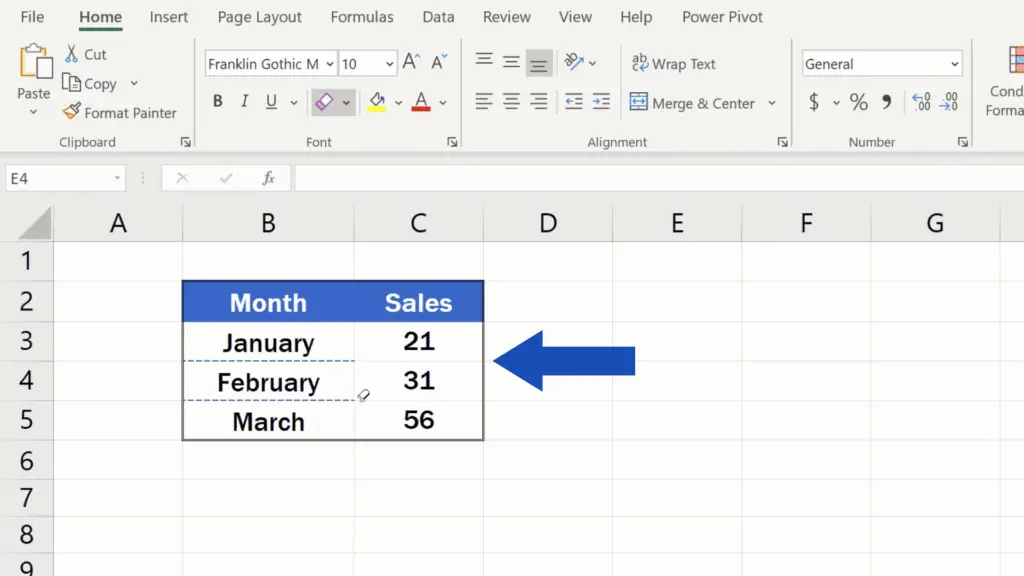
The first one we’re gonna talk about helps you remove the border only partly. Go to the Border options, select ‘Erase Border’ and click on a border line you want to erase. And it’s gone! Once finished, press the Escape button to exit the ‘eraser’ mode.

How to Remove All Borders at Once

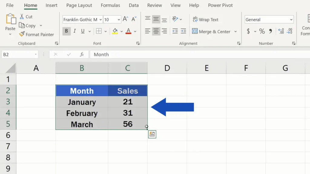
And here comes the second one, which is the most effective way to remove all borders at once. Select the area where you want to remove the borders. From the options, select ‘No Borders’.

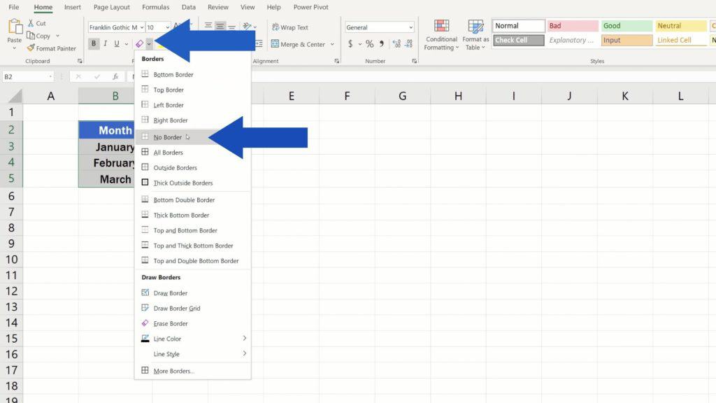
Voila! All borders from the selected area have been removed!

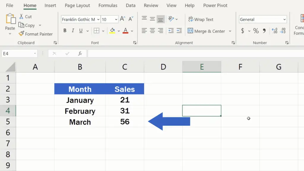
Now you might also be curious how to get rid of the gridlines in a spreadsheet. If you want to know more, we’re happy to help! Learn how to hide gridlines in Excel in another of the tutorials by EasyClick Academy. The link’s in the list below.

Don’t miss out a great opportunity to learn:

• How to Hide Gridlines in Excel (the Easy Way)
• How to Insert Column in Excel
• How to Delete Sheet in Excel

If you found this tutorial helpful, give us a like and watch other tutorials by EasyClick Academy. Learn how to use Excel in a quick and easy way!

Is this your first time on EasyClick? We’ll be more than happy to welcome you in our online community. Hit that Subscribe button and join the EasyClickers!

Thanks for watching and I’ll see you in the next tutorial!