How to Link Cells in Different Excel Spreadsheets (In One or More Excel files)

In this tutorial, we’re gonna go through how to link cells in different Excel spreadsheets. You’ll be able to use data from a different spreadsheet located within the same workbook, in a single file, but also from a spreadsheet which is a part of a completely different Excel file.

Ready to crack on?

Would you rather watch this tutorial? Click the play button below!

How to Link Cells within a Single Workbook

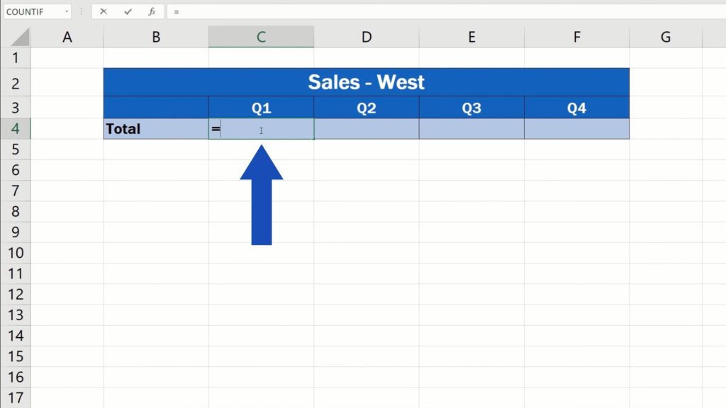
To link cells within a single workbook, you need to select the cell where you’d like to show the information from the other spreadsheet first.

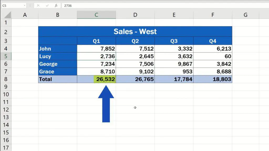
Here we’ll click into C4, which is the cell where we want to display the sales for Quarter 1. Let’s enter the equal sign, and now we need to open the spreadsheet with the information we want to show in this cell. So, we’ll go down here and click on the sheet ‘Sales-West’, which contains all the details of the western region sales for individual quarters.

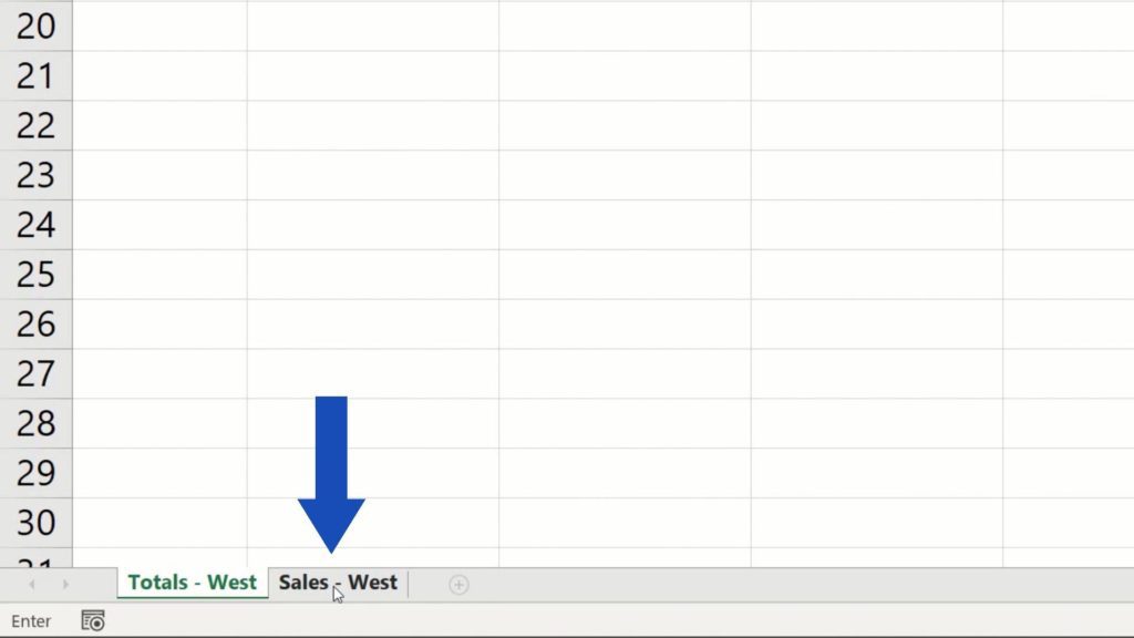
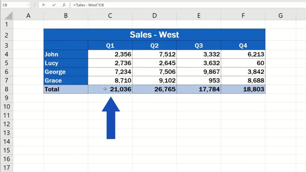
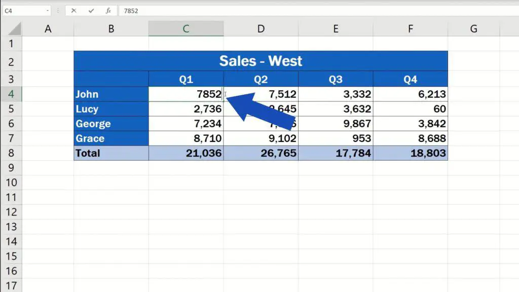
Since we want to show only the total for Quarter 1, we’ll click on the cell C8, press Enter and that’s it!

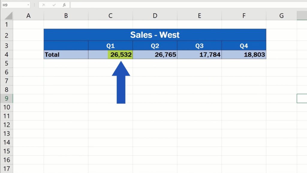
The cell C4 in the spreadsheet ‘Totals-West’ shows the data from the spreadsheet ‘Sales-West’.

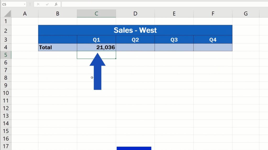
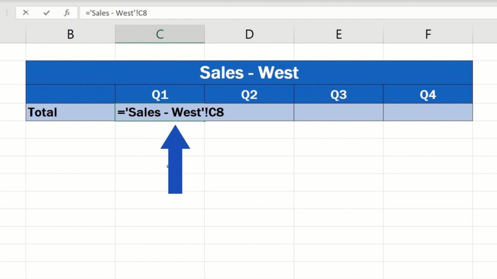
If we click into the cell C4 now, we can see the formula behind this link that Excel’s made. There’s the equal sign, and after that Excel uses single quotation marks with the spreadsheet name from which we’re taking the data – Sales-West. Then there’s an exclamation mark followed by the coordinates of the cell that contains the information we’re using, which is C8.

How to Copy the Link Formula through the Rest of the Quarters

Here’s one thing worth mentioning though. There’s a little trick which can help you transfer data from other quarters from the spreadsheet ‘Sales-West’ to the rest of the cells in this row in no time at all.

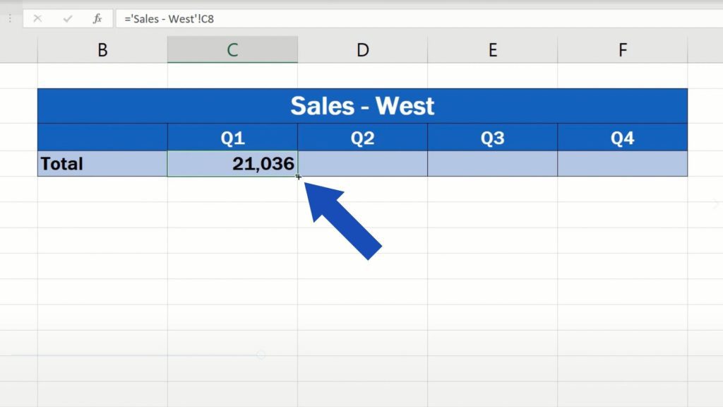
The link can simply be copied by dragging the lower right corner of the cell where we’ve already got the formula through the rest of the quarters.

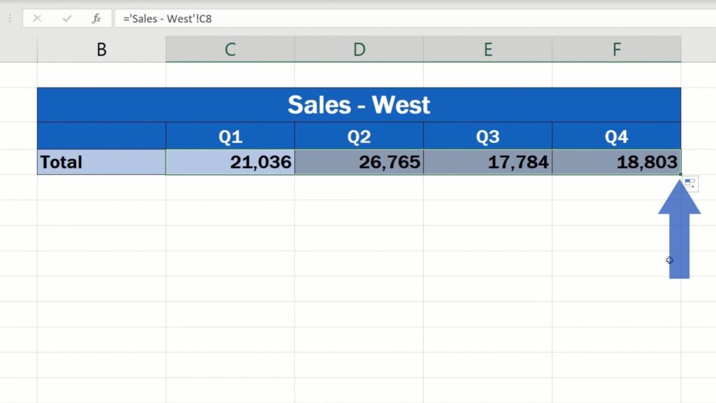
Of course, the formulas with the links works dynamically, which means if we make a change in the spreadsheet ‘Sales-West’, for example, we’ll change John’s sales figure for Quarter 1, the total of sales for Quarter 1 will update and this change will be reflected in the sheet containing the link – ‘Totals-West’.

Now, let’s move on and have a look at how to link cells in different spreadsheets located in separate Excel files.

How to Link the Cells in Different Spreadsheets Located in Separate Excel Files

As an example, we’ll use this folder with three different Excel files – the files with the sales figures for the region West and East and the file for Totals that summarises all data.

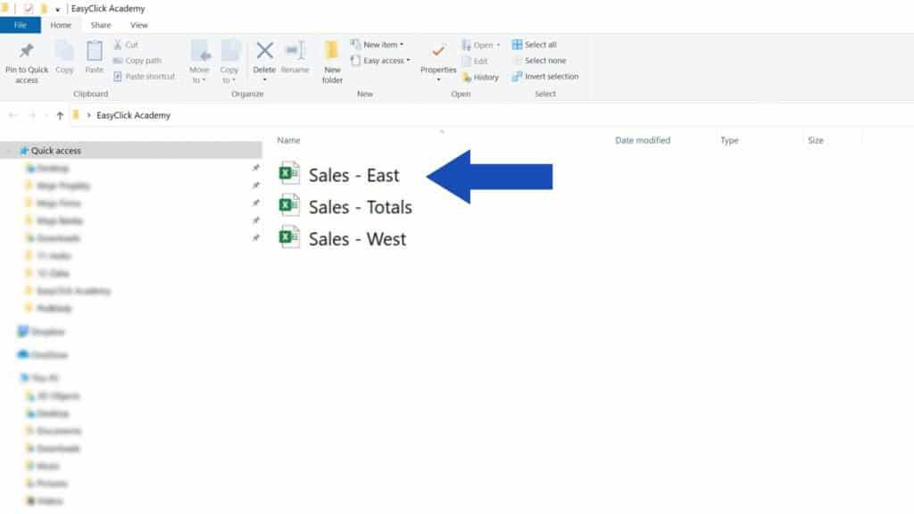
Let’s open all three of them at once and let’s click into the file containing the totals for all sales. In this spreadsheet, we’re gonna make links to the data from both regions for all four quarters stored in separate Excel files.

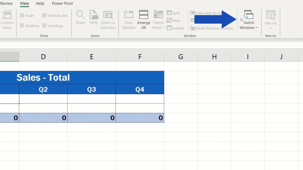
To do that, click into the selected cell, enter the equal sign, but to make links to a different Excel file, you need to go to the tab View and select the option ‘Switch Windows’.

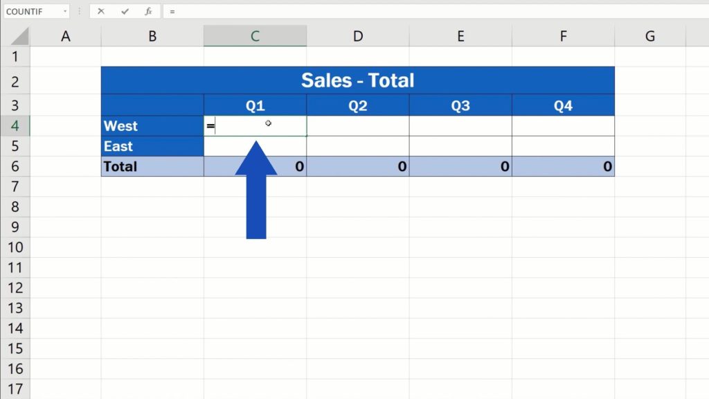
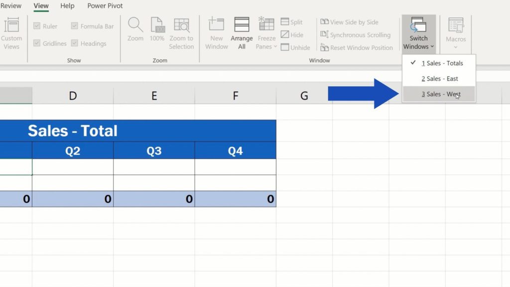
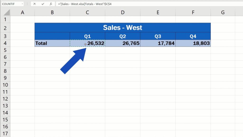
You’ll be provided with the list of currently opened files. Select ‘Sales-West’ to view this workbook. Here we want to use the data for Quarter 1, so click on the cell C4, press Enter and here we go!

Excel navigated back to the file ‘Sales-Totals’ and included the Q1 value from the file ‘Sales-West’ into the cell C4, just as we wanted.

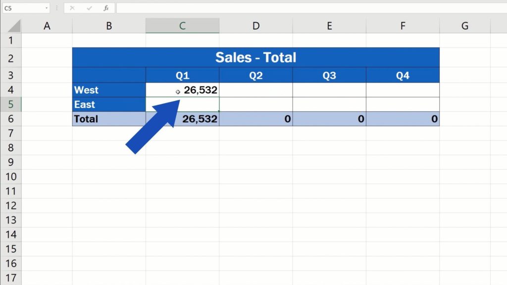
Let’s just give it a quick check.

When we click into C4 and have a look at the formula, we’ll see how Excel makes links between two files. It’s slightly different from what we did a while ago when we made links within one workbook. First, there’s the equal sign, but after that, there comes the file name in square brackets along with the name of the sheet, all within single quotes, followed by the reference to the cell containing the information we want to display here.

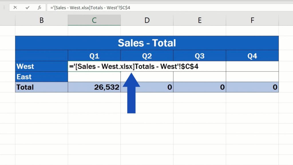
However, if we wanted to copy this formula through all quarters here, we wouldn’t be successful. You can see that the reference to the cell C4 contains these dollar signs. This means that the cell reference is absolute – it’s fixed and the copied formulas would contain the reference only to this particular cell, which we actually don’t want.

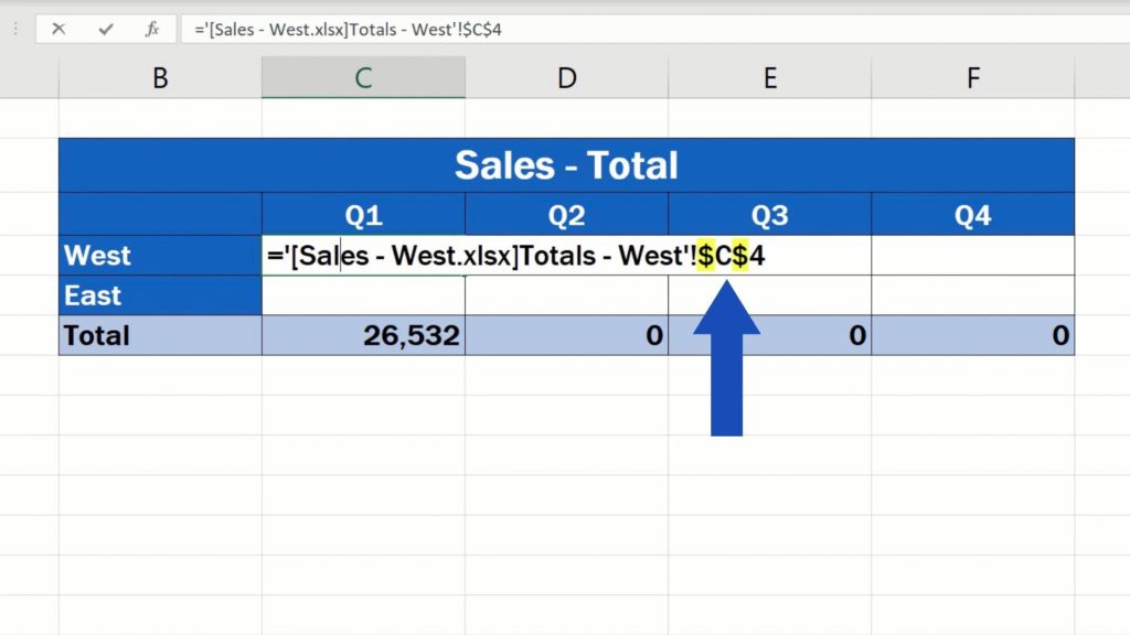
For now, we’ll remove these dollar signs and if you’d like to know more on how an absolute cell reference works, you can have a look at the tutorial on how to use absolute cell reference in Excel. We’ve included the link to this tutorial in the list below.

Once we’ve removed the dollar signs, we can press Enter and copy the formula by dragging the lower right corner of the cell across all quarters.

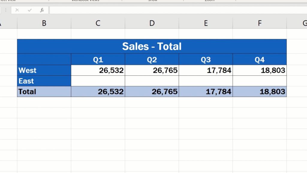
And we can repeat these steps to transfer the data from the file ‘Sales-East’ to the file with the totals. Like this.

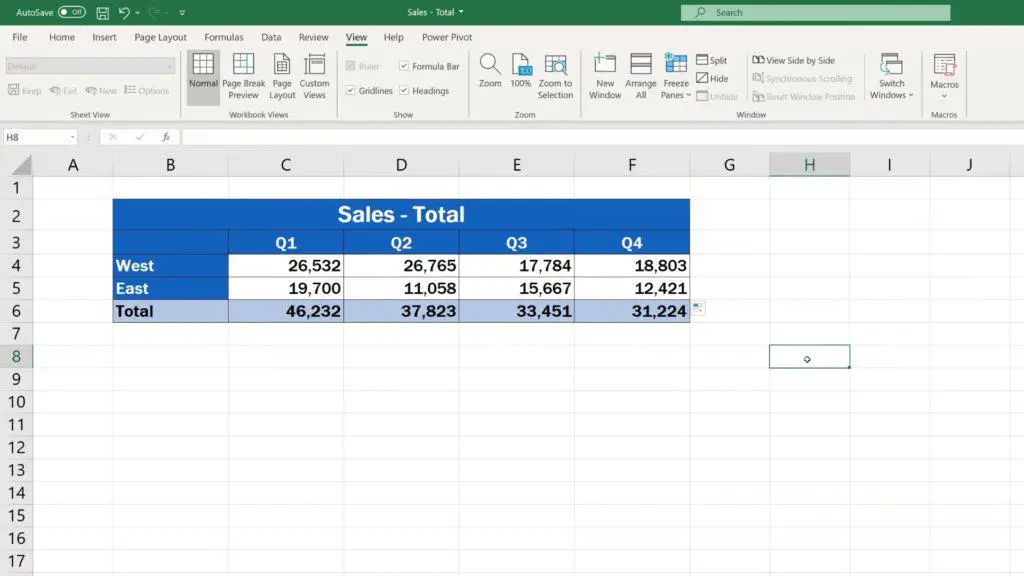
There we go!

We’re quite sure you’ll find these two simple and easy ways to link cells in different Excel spreadsheets handy and helpful.

Don’t miss out a great opportunity to learn:

• How to Use Absolute Cell Reference in Excel
• How to Delete Sheet in Excel
• How to Rename Sheet in Excel
• How to Hide Sheets in Excel

If you found this tutorial helpful, give us a like and watch other tutorials by EasyClick Academy. Learn how to use Excel in a quick and easy way!

Is this your first time on EasyClick? We’ll be more than happy to welcome you in our online community. Hit that Subscribe button and join the EasyClickers!

Thanks for watching and I’ll see you in the next tutorial!