How to Insert Bullet Points in Excel (Quick and Practical Solution)

In this video tutorial, we’ll be having a look at a quick and practical solution to how to insert bullet points in Excel.

Let’s not waste any time and get straight into it!

Would you rather watch this tutorial? Click the play button below!

There are multiple ways how to insert bullet points in Excel and today, we’re gonna go through the easiest, most practical one.

How to Insert Circle Bullet Points in Excel

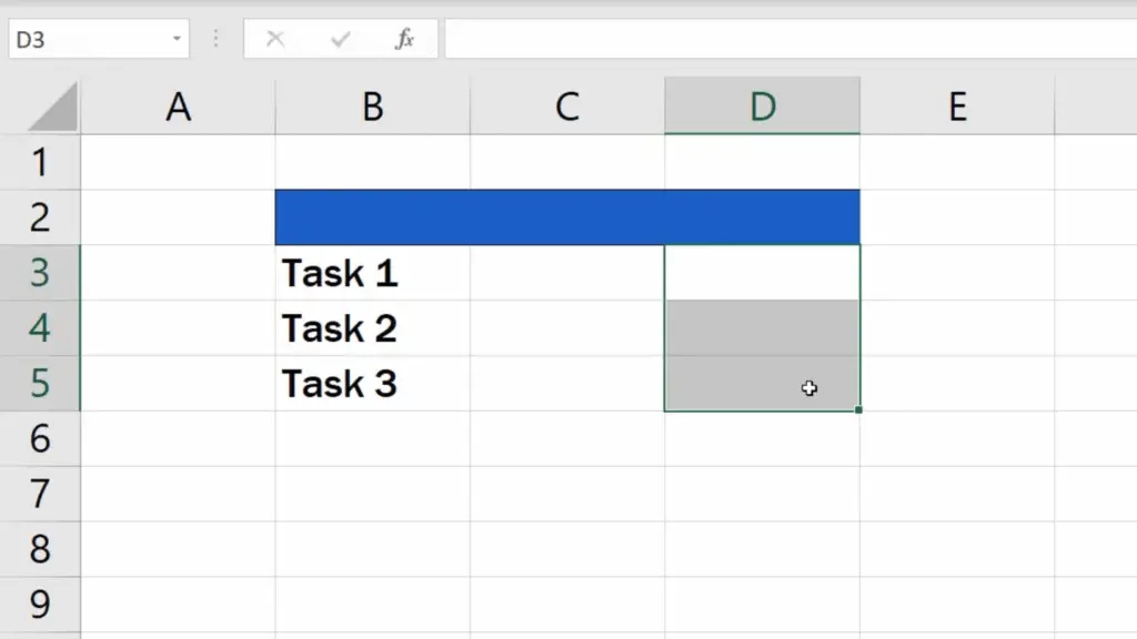
Let’s say we want to display the list of these three tasks from the table using bullet points in column D. First, we’ve got to select the cells where the list with bullet points will display.

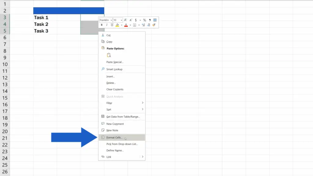
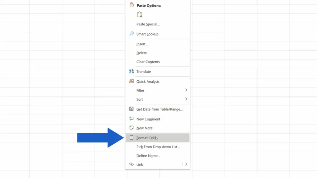
Then, through a right-click, we access the option ‘Format Cells’.

In the tab ‘Number’, we need to select the category ‘Custom’.

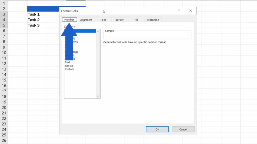
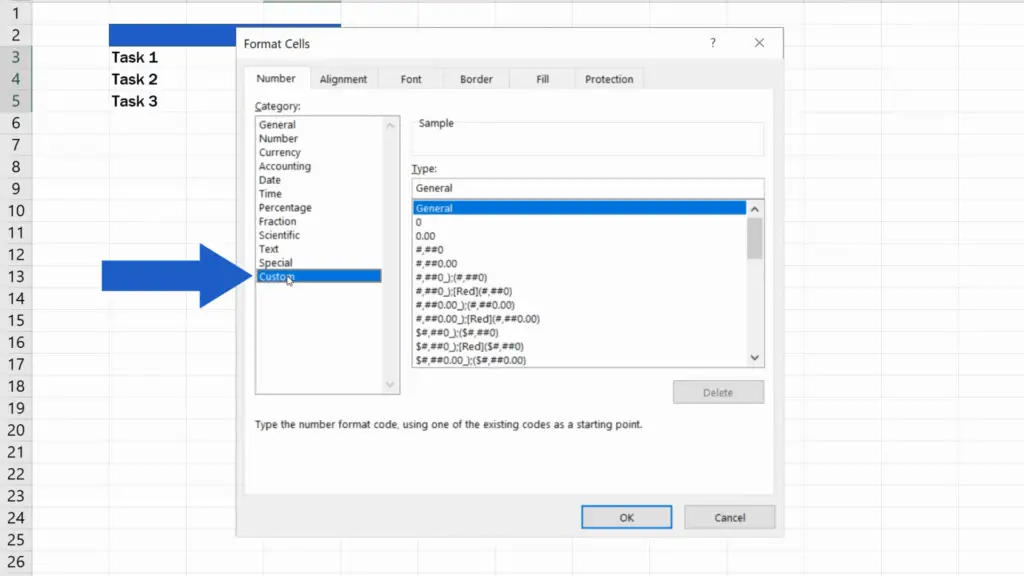
Now, what follows is crucial to getting our bullet points to display with the task list.

To insert bullet points in the cells, start with entering the specific bullet point symbol you want to use here, in this field, and add a space followed by the at sign.

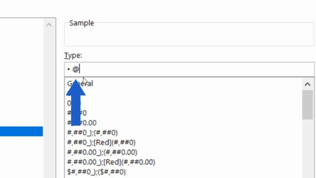
Once done, press OK and let’s try it out together!

When we type in ‘Task 1, 2, 3’, Excel inserts the bullet point we entered in the ‘Type:’ field a short while ago in front of each entry.

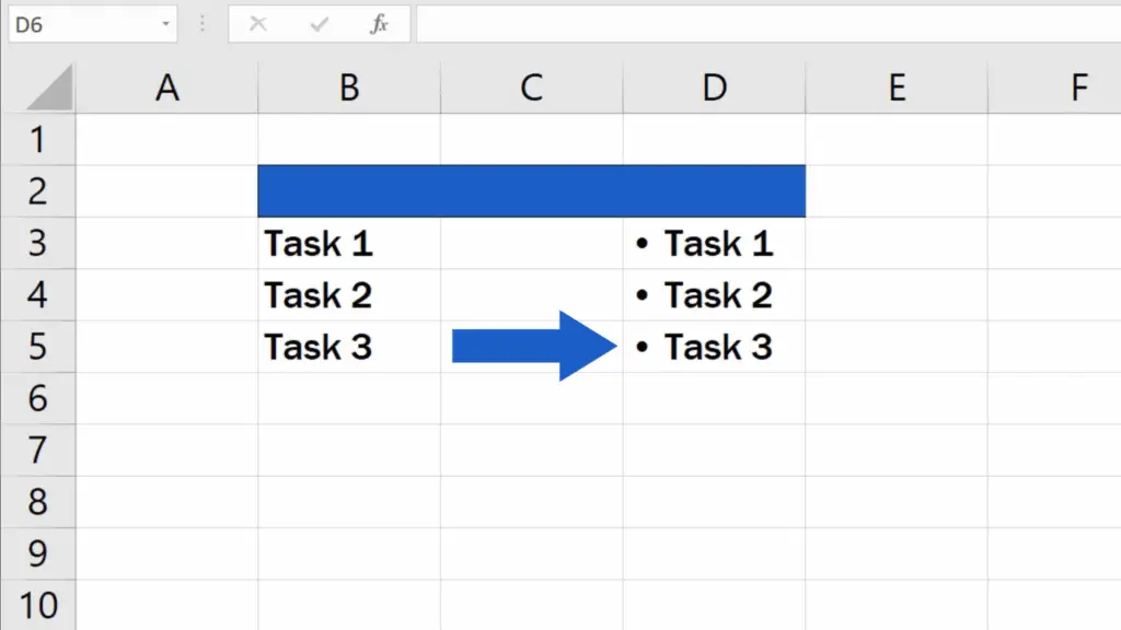
To change the type of the bullet point is actually child’s play. Let’s have a look and see.

How to Insert Empty Bullet Points in Excel

Just as we started a while ago, we need to select the cells where we want to make changes.

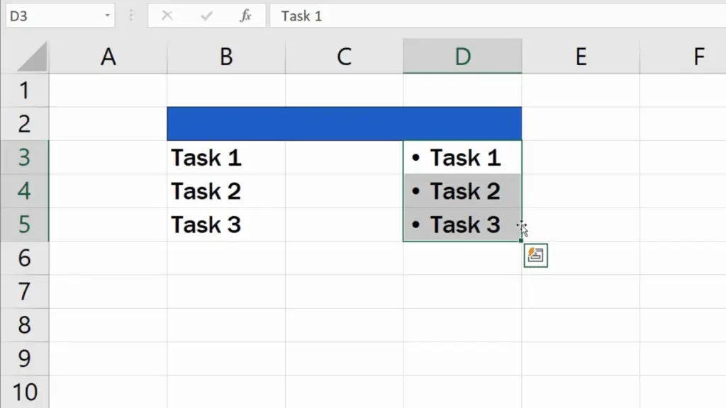
Through a right-click we choose ‘Format Cells’ and in the field ‘Type:’ we need to insert the symbol we want to use.

For example, now instead of the circle bullet point, we want to use an empty bullet point, so we’ll enter it here.

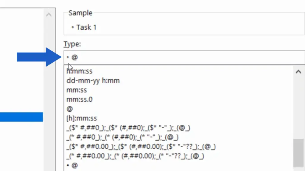
Of course you can use any type of bullet point or any symbol you like. So, we’re gonna go for the empty bullet point now. If you need, you can find this combination of bullet points in the list below, so that you could copy and paste it conveniently anytime.

• @
◦ @

Once we’ve inserted the chosen symbols, we press OK and Excel adds these bullet points to the text within the selected cells.

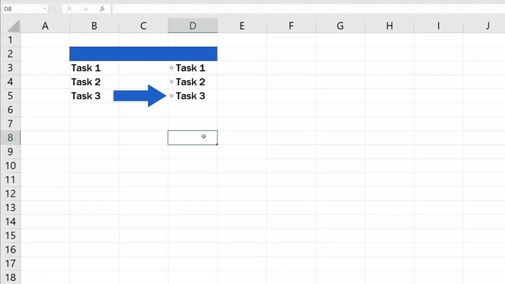
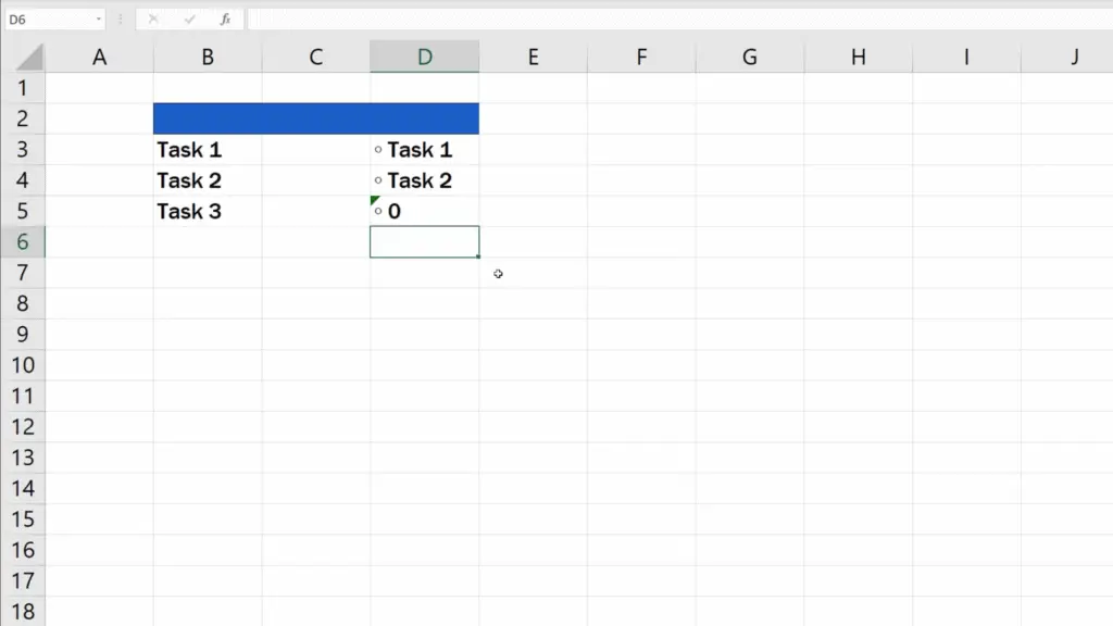
And even if you change the information in the table, the selected bullet points will keep displaying in the cells formatted this way.

Don’t miss out a great opportunity to learn:

• How to Insert a Symbol in Excel
• How to Insert Image in Excel Cell (Correctly)
• How to Insert Comment and Note in Excel

If you found this tutorial helpful, give us a like and watch other tutorials by EasyClick Academy. Learn how to use Excel in a quick and easy way!

Is this your first time on EasyClick? We’ll be more than happy to welcome you in our online community. Hit that Subscribe button and join the EasyClickers!

Thanks for watching and I’ll see you in the next tutorial!