How to Insert a Watermark in Excel (Picture or Text)

Today’s tutorial will be on how to insert a watermark in Excel. We’re going to go through a quick and easy way to do that, and we’ll be talking about pictures as well as text.

Get ready, we’re about to start!

Would you rather watch this tutorial? Click the play button below!

How to Insert a Watermark in Excel

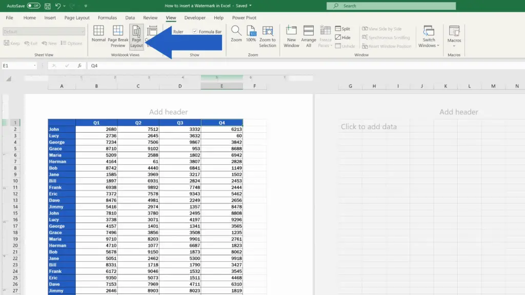
To insert a watermark in an Excel spreadsheet, go to the ‘Page Layout’ view on the View tab.

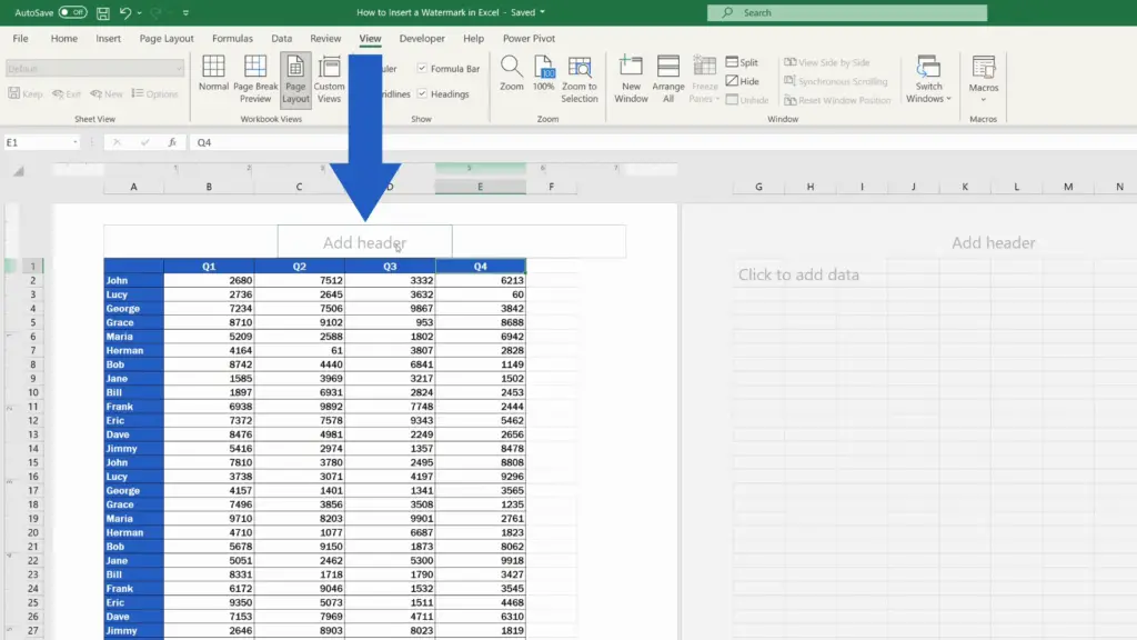
Then click on ‘Add header’, which will open the header section of the document. So basically, we’ll use the header to insert a picture or text as a watermark.

How to Add a Picture Watermark Properly

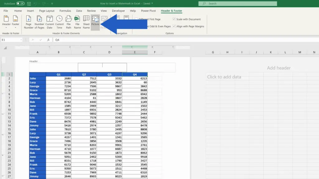
Let’s have a look at how to add a picture watermark – we need to be in the Header & Footer tab where we select ‘Picture’.

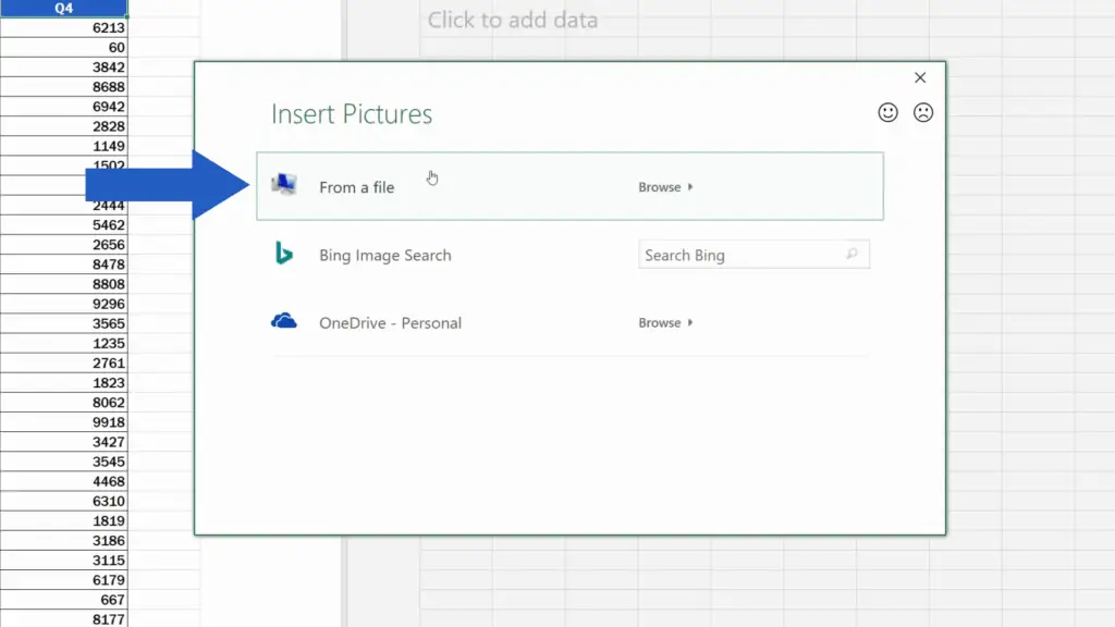
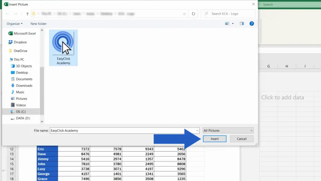
Now you’ll see a window with multiple options to insert the picture. We’ll use the first one – from a file. Let’s click on it and browse the computer to find the picture we’ve prepared. Select the picture and confirm by clicking on Insert.

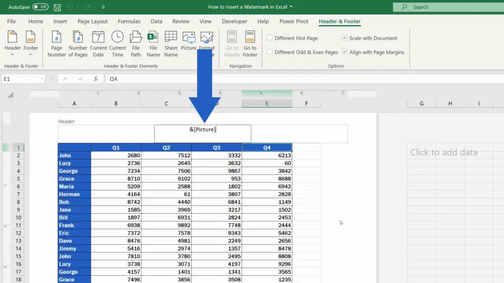
You can notice that Excel shows a piece of text instead of the picture, so to see the picture itself, click anywhere on the sheet and you’ll be able to see the inserted picture, which seems to be way too big though.

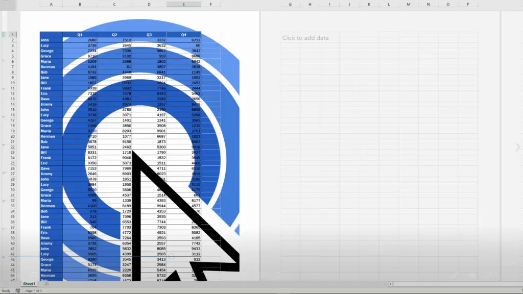
Let’s fix this and format the picture together.

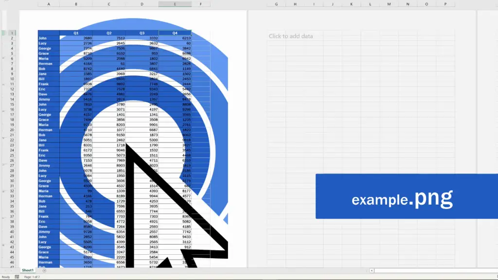
But before we move to that, it’s important to note that the best format for a picture watermark is PNG and it might be a good idea to prepare the picture as a logo with a transparent background, for example.

How to Format a Picture Watermark

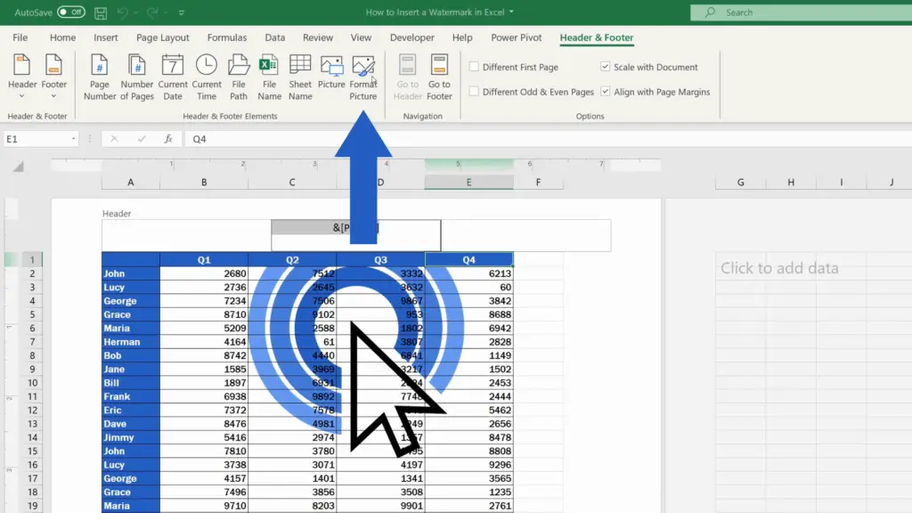
To format the picture, we need to click into the header again to open the Header & Footer tab where we click on ‘Format Picture’. Here we can find some options that might help us modify the picture as we need.

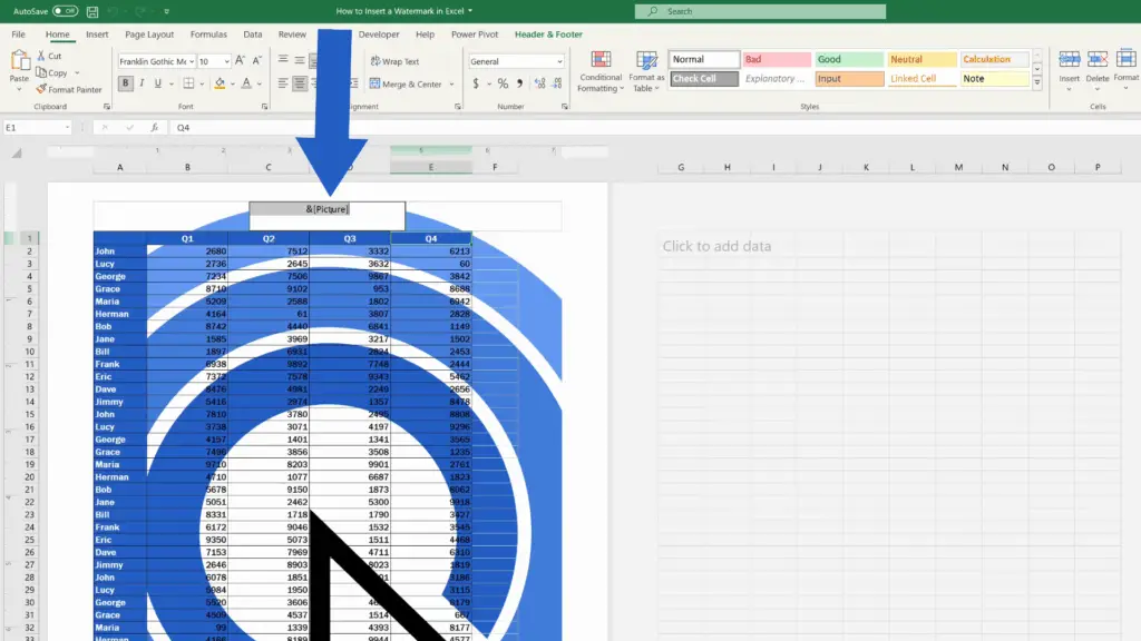
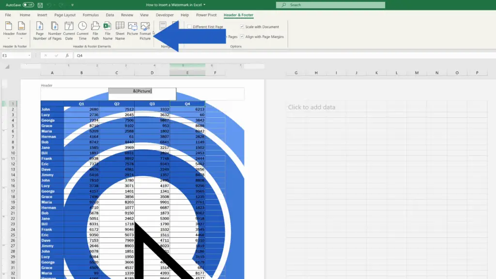
First, I would suggest resizing the picture. We can use a specific number to set the height and the width or simply use percentage under ‘Scale’.

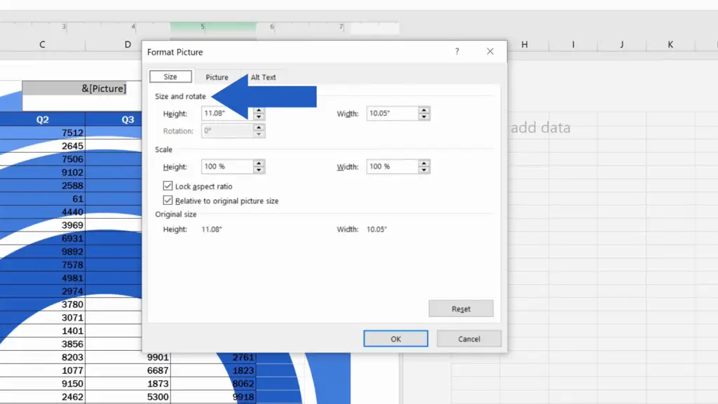
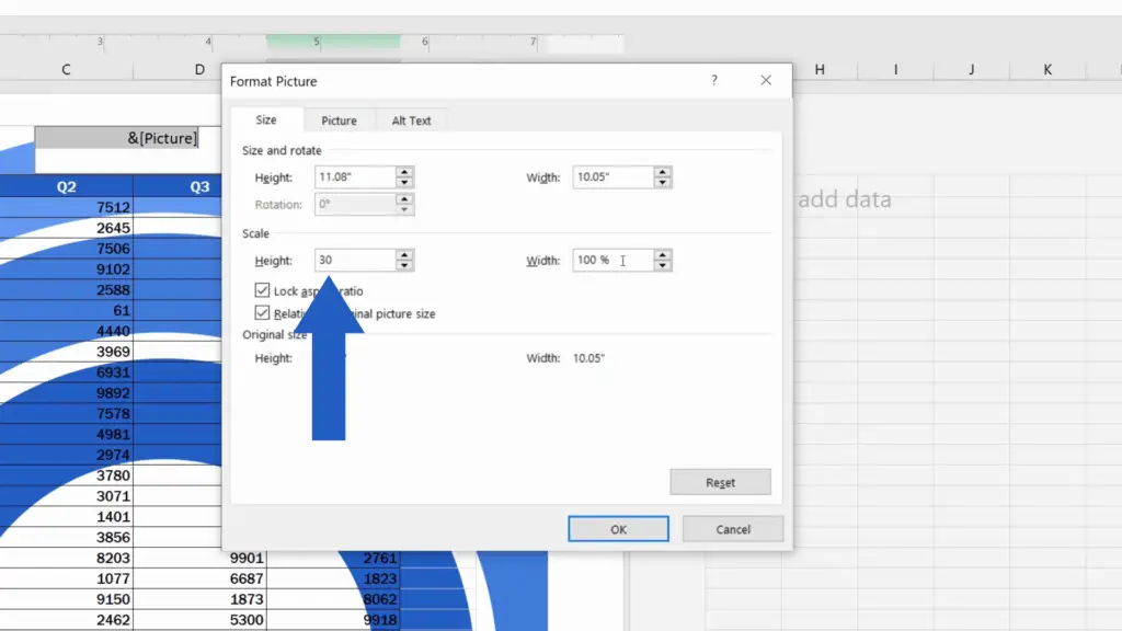
Here we’ll set the percentage to 30% and after clicking on OK, you can see that the picture is much smaller, which is more convenient for us.

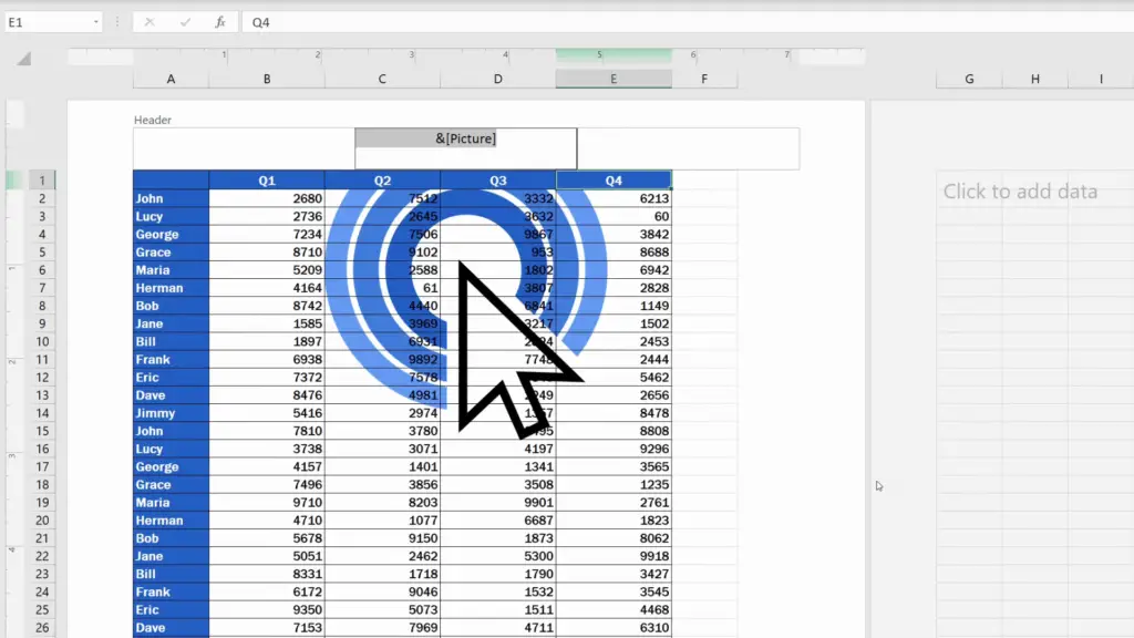
Now, let’s make some more changes – let’s go back to ‘Format Picture’, go to the tab ‘Picture’ and we’re going to change the picture colour.

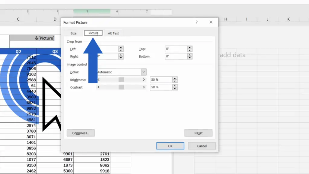
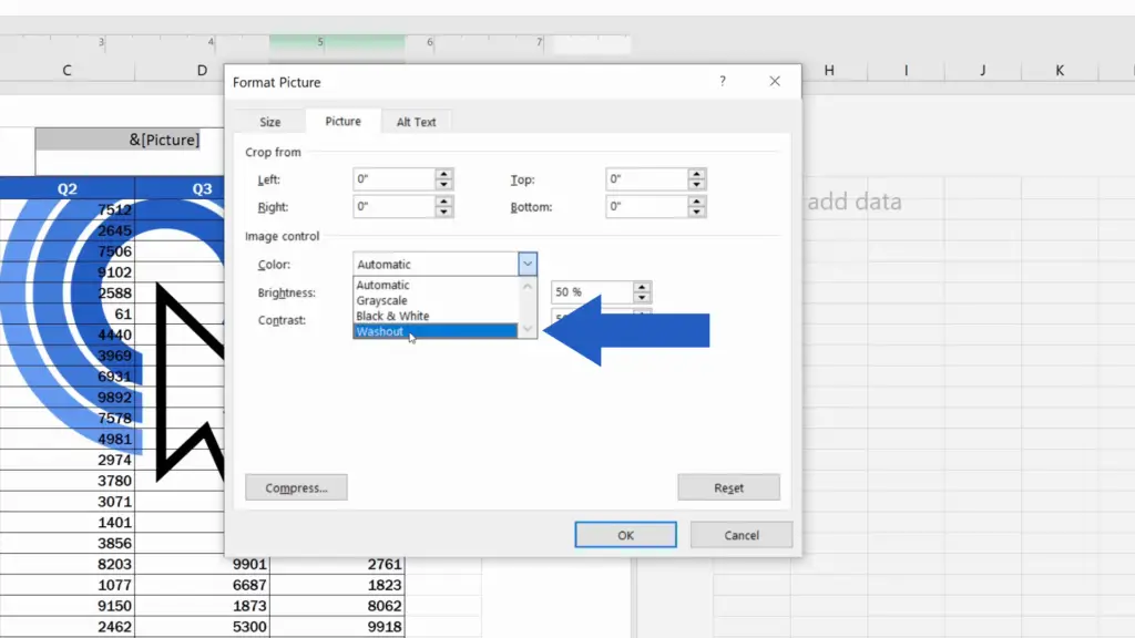
As you can see, there are more options we can use, so now we’ll go for ‘Washout’, confirm with OK and our picture looks more like a watermark now.

But that’s not all.

We need to move the picture down a little bit. So, we click into the header again and press Enter as many times as needed until the picture location is just as we want it to be. We’ll place it here.

To remove the watermark, click into the header section, select all that’s there and use the key ‘Delete’. There you go! The watermark’s gone.

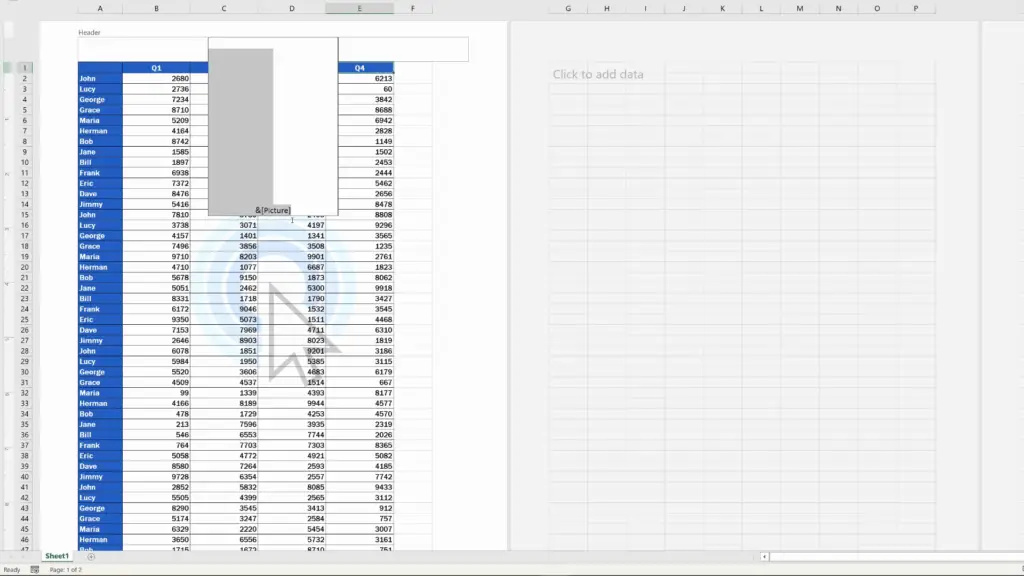
Now let’s move on and have a look at how to insert a text watermark.

How to Insert a Text Watermark

Click into the header again and simply type in whatever text you want to use as a watermark. We’re going to use the word ‘DRAFT’ here.

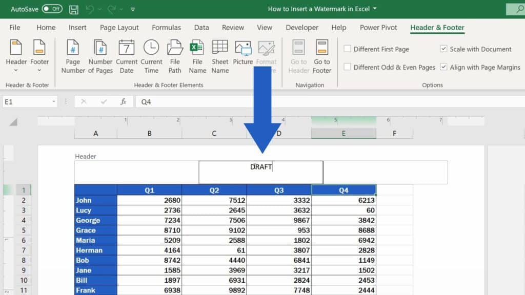
Next, we’re going to select the text to do some useful formatting.

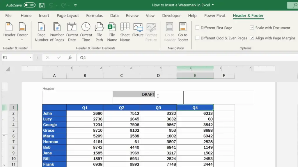
For example, in the Home tab, we can choose a font type – let’s say we’re going to use Arial Black here.

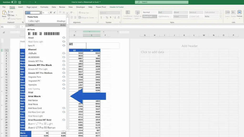
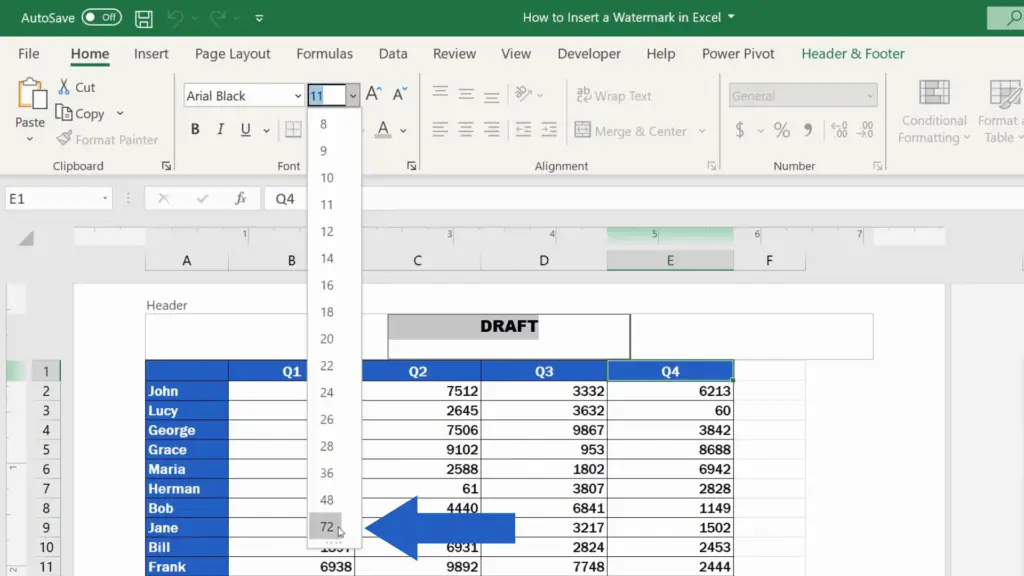
Also, the size of the text can be adjusted here, so this will be font size 72.

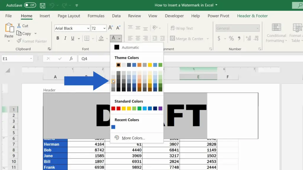
Apart from that, we can select the colour of the text, let’s say we’ll go for this grey.

And just as with the picture, even here we can use the key ‘Enter’ to find the right place for the watermark.

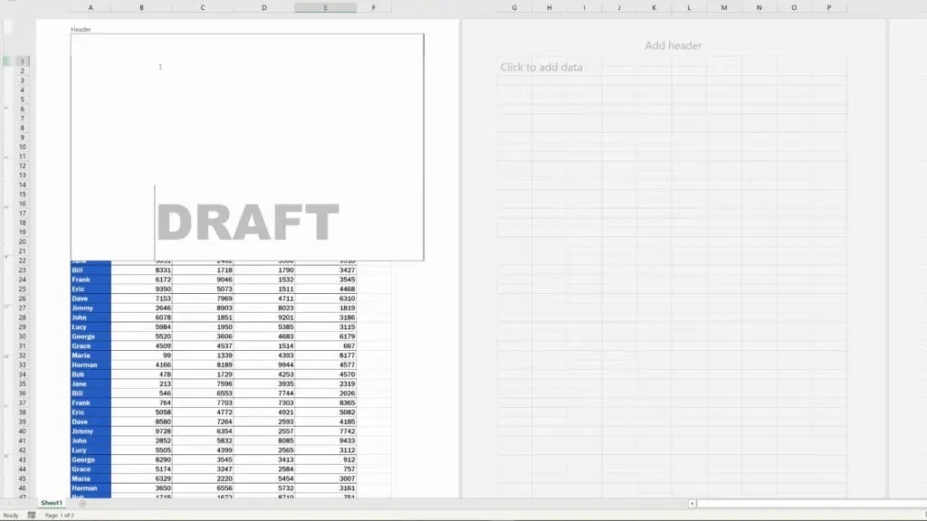
And that’s about it. If we click anywhere on the spreadsheet, we’ll see our watermark in all its beauty 😊

If, for some reason, you need to remove it, you can do it the same way as with the picture.

Don’t miss out a great opportunity to learn:

• How to Insert a Checkbox in Excel (Quick and Easy)
• How to Insert Image in Excel Cell (Correctly)
• How to Insert Comment and Note in Excel

If you found this tutorial helpful, give us a like and watch other tutorials by EasyClick Academy. Learn how to use Excel in a quick and easy way!

Is this your first time on EasyClick? We’ll be more than happy to welcome you in our online community. Hit that Subscribe button and join the EasyClickers!

Thanks for watching and I’ll see you in the next tutorial!