How to Highlight Duplicates in Excel (Super Easy)

In this tutorial we’re going to have a look at how to highlight duplicates in Excel in a column, multiple columns or, if needed, throughout a data table of any size.

Let’s begin!

How to Highlight Duplicates

To highlight duplicates, first we need to select the relevant area.

Here, we’re going to begin with one column – in our case it’ll be column B, the column containing names. Let’s click on the letter B here in the column header and the whole column is highlighted.

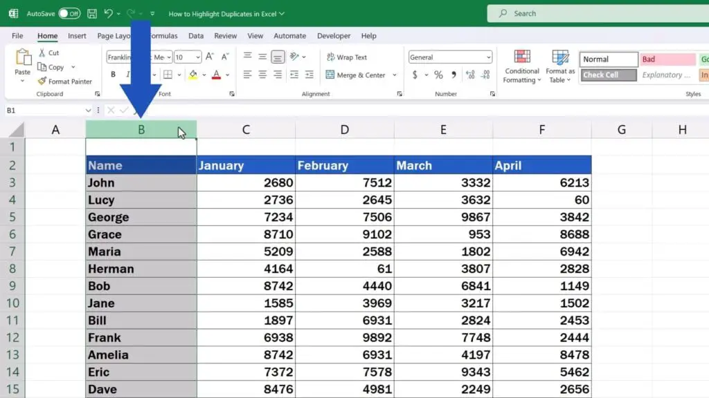
The same way we can extend the selection through two or more columns or wherever we’d like to select cells for highlighting duplicates.

Now we’ll work with one column only, so let’s select column B and let’s move on.

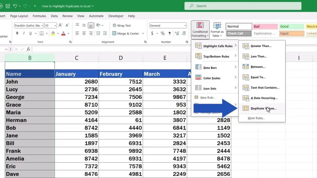
Once selected, we can highlight duplicates in the column by finding the section ‘Styles’ and clicking on ‘Conditional Formatting’. Then we carry on to ‘Highlight Cells Rules’ and eventually select ‘Duplicate Values’.

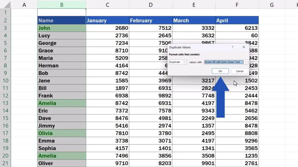
All duplicated values in column B have been highlighted – here we’ve got names John, Amelia, and Olivia.

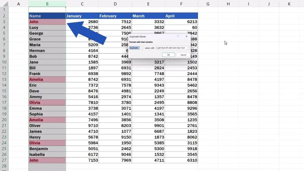
At the same time, a window has appeared where we can customise the highlighting.

How to Highlight Unique Values

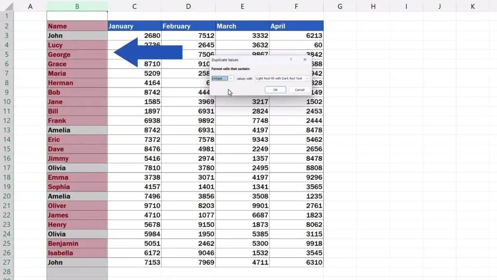
If we’d like to highlight unique values in the same column, we can simply switch from ‘Duplicate’ to ‘Unique’ right here.

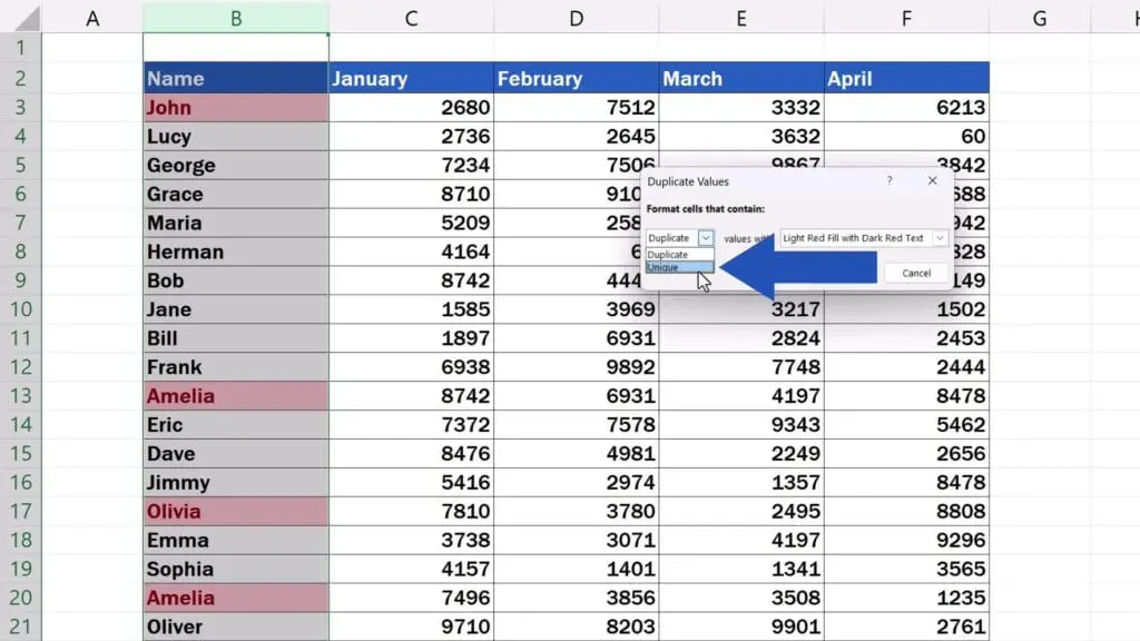
And here we go! Here are all unique values highlighted in column B.

How to Change the Colour Formatting of the Highlighted Values

Let’s switch back to ‘Duplicate’ and take a look at how we can change the colour formatting of the highlighted values.

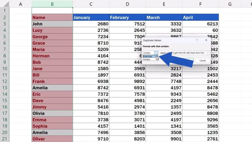
We can have them highlighted in red like this, or yellow like this, or even green, or we can pick whichever option here suits us best.

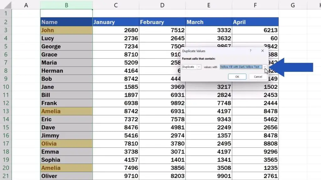
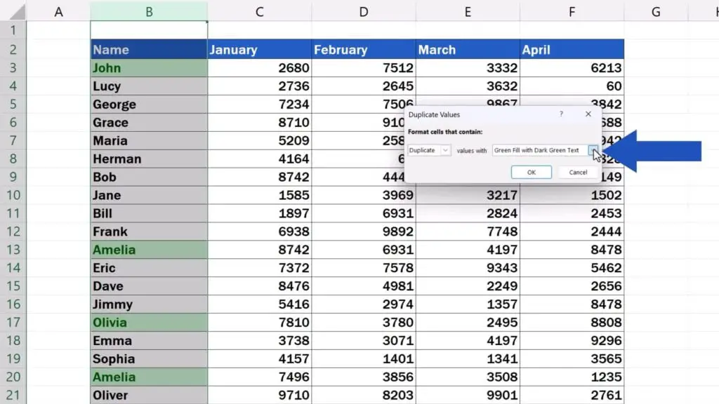
As soon as we pick the colour, we confirm with ‘OK’ and the duplicates get highlighted in the style we’ve chosen.

Now let’s see how we can remove the highlighting.

How to Remove the Highlighting

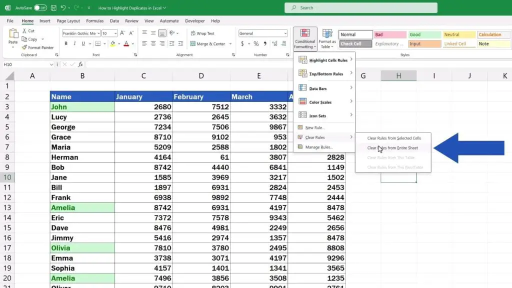
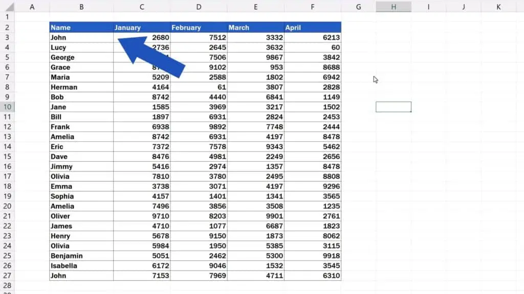
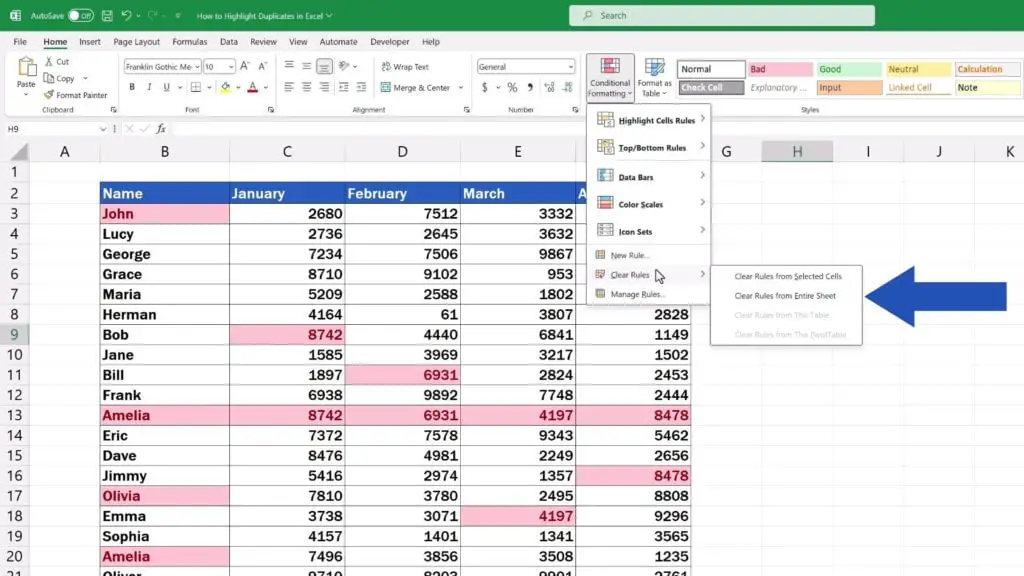
Again, we go to the section ‘Styles’, click on ‘Conditional Formatting’ and find ‘Clear Rules’. Here we can decide to ‘Clear Rules from Selected Cells’ or ‘from Entire Sheet’. We’ll go for the entire sheet now because that way we don’t need to select any part of the spreadsheet and the highlighting will be completely removed.

And finally, we’ll have a look at one last thing.

How to Highlight Duplicates Throughout the Data Table

To highlight duplicates throughout the data table, we need to select the whole table. We can do it by clicking here, on the upper left-hand corner to select the whole sheet, which includes the data table.

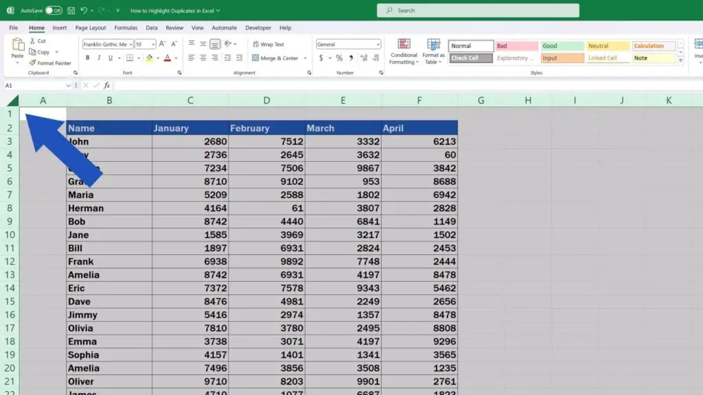
Then we follow the same steps as before.

We go to ‘Styles’, select ‘Conditional Formatting’, click on ‘Highlight Cells Rules’ and then click on ‘Duplicate Values’.

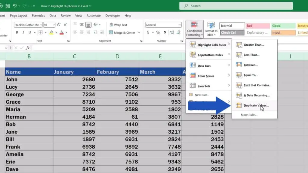
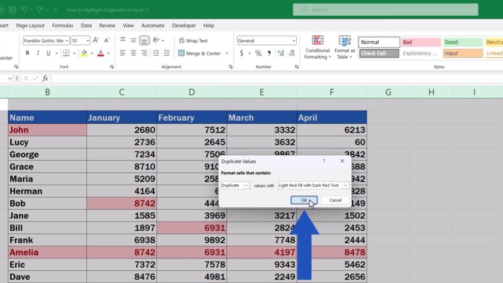
We’ll keep the default colour for highlighting, hit ‘OK’ and that’s it! Duplicates have been highlighted throughout the table!

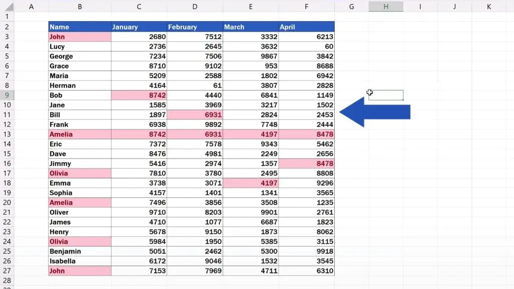
To remove the highlighting, again, click on ‘Conditional Formatting’, then ‘Clear Rules’ and finally ‘Clear Rules from Entire Sheet’, which will remove the highlighting across the data table.

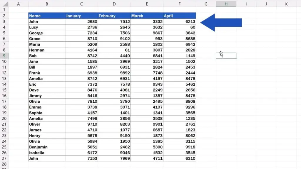
Following the same steps, we can highlight duplicates in one or multiple columns or throughout a data table.

If you’d like to know how to remove duplicates from a data table, check out another tutorial by EasyClick Academy. You can find the link in the list below.

Don’t miss out a great opportunity to learn:

• How to Remove Duplicates in Excel
• How to Find Duplicates in Excel
• How to Count Unique Values in Excel (Quick and Easy)

If you found this tutorial helpful, give us a like and watch other tutorials by EasyClick Academy. Learn how to use Excel in a quick and easy way!

Is this your first time on EasyClick? We’ll be more than happy to welcome you in our online community. Hit that Subscribe button and join the EasyClickers!

Thanks for watching and I’ll see you in the next tutorial!