How to Hide Gridlines in Excel (the Easy Way)

In this short tutorial you’ll see the easiest way how to hide gridlines in Excel, either in the whole spreadsheet or in a selected area.

Ready to start?

Would you rather watch this tutorial? Click the play button below!

How to Hide Gridlines in the Whole Spreadsheet

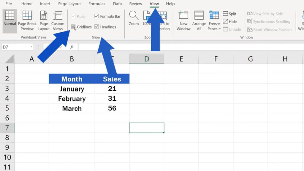
f you want to hide gridlines in the whole spreadsheet, simply click on View tab, go to the section Show and unselect the option Gridlines.

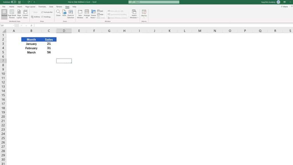
The gridlines immediately disappear from the whole spreadsheet and the area looks nice and clean.

How to Show Gridlines in Excel

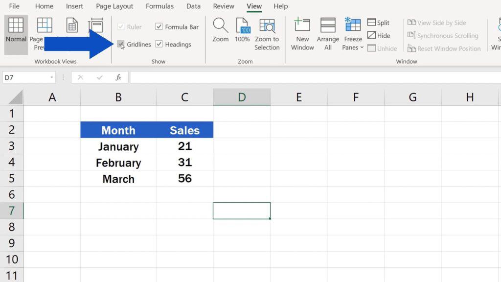
In case you need the gridlines to be visible in the sheet, you can simply select the option Gridlines and they’ll be back on, making it easy to navigate through the cells.

How to Hide Gridlines in a Selected Area

Now, you might wonder – what if I need to remove gridlines only in a selected area of the spreadsheet? This little tip will do the trick!

Let’s say we don’t want gridlines to appear in the data table.

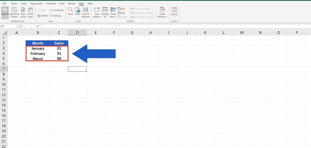
We select the area of the table, go to Home tab and use the function ‘Fill Color’ to change the background colour of the area to white.

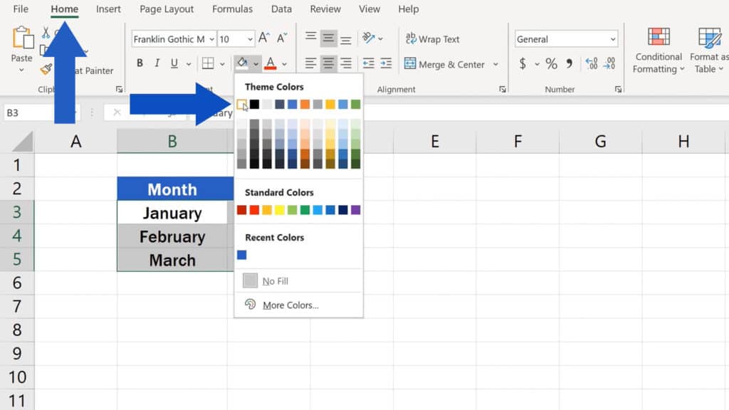
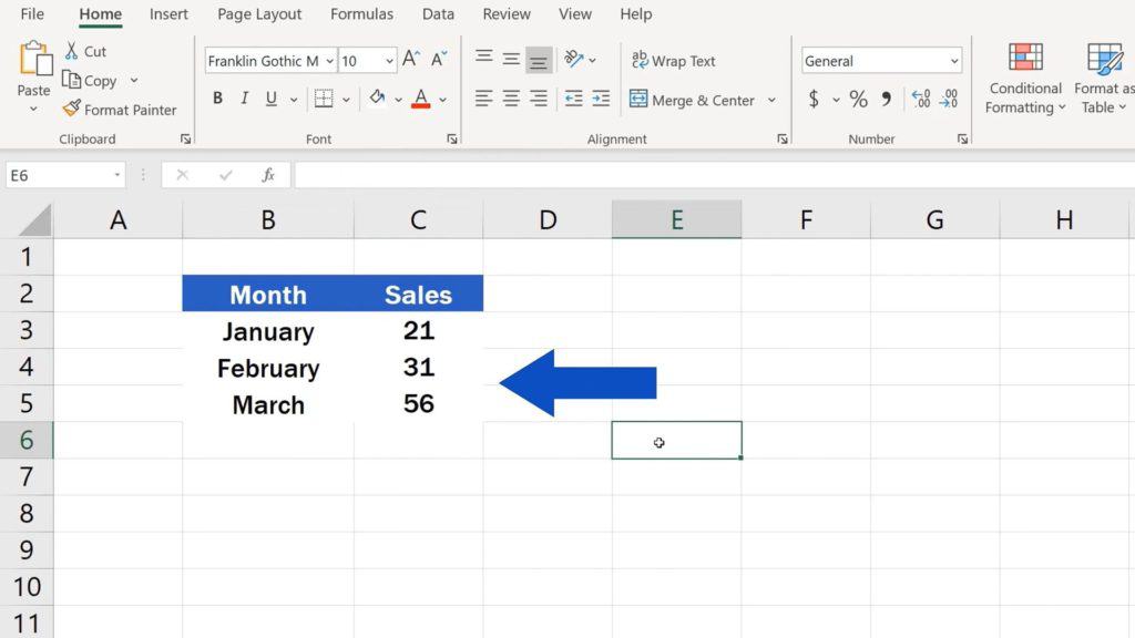
Thanks to this, no gridlines are now visible in the area we’d selected!

Don’t miss out a great opportunity to learn:

• How to Show or Hide the Ribbon in Excel
• How to Show or Hide the Formula Bar in Excel (Quick and Easy)
• How to Use the VLOOKUP Function in Excel
• How to Move Columns in Excel (The Easiest Way)

If you found this tutorial helpful, give us a like and watch other video tutorials by EasyClick Academy. Learn how to use Excel in a quick and easy way!

Is this your first time on EasyClick? We’ll be more than happy to welcome you in our online community. Hit that Subscribe button and join the EasyClickers!

Thanks for watching and I’ll see you in the next tutorial!