How to Hide Formulas in Excel (Quick and Easy)

This tutorial offers a quick and easy way how to hide formulas in Excel. Thanks to these set of steps no one will be able to see the formulas you used in a data table.

Ready to start?

Would you rather watch this tutorial? Click the play button below!

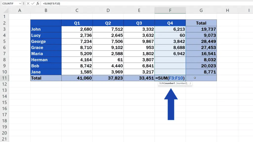
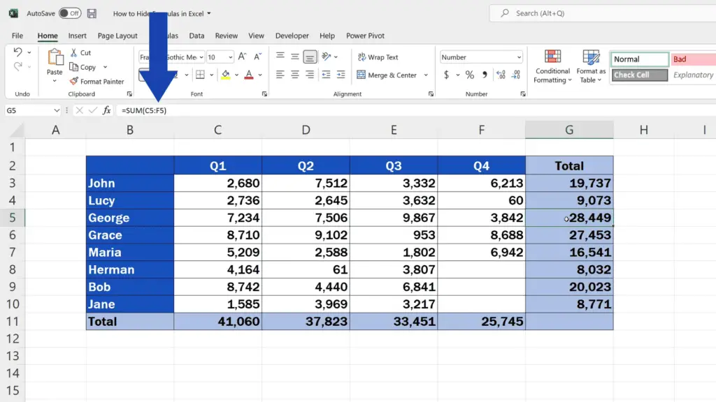
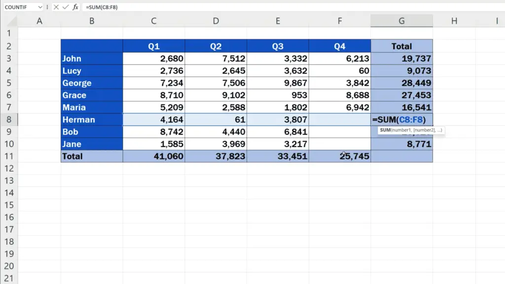
If there are any formulas in a data table, it’s quite easy to spot them – just click into the cell containing a formula and you can see it right away. Or have a look at the formula bar here at the top. If you don’t want anyone to see the formulas, you can hide them using the following steps.

How to Hide Formulas in Excel

First, select the cells which contain the formulas you want to hide. Then use the right-click to select ‘Format Cells’.

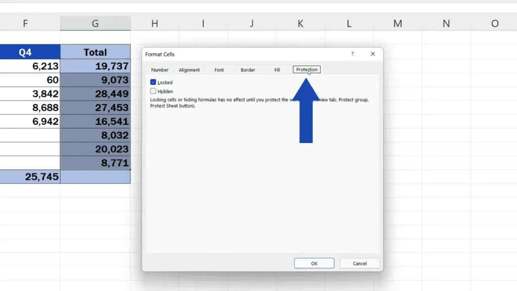
You’ll see a window where you can go to the tab Protection. Select the option ‘Hidden’, which practically hides the contents of the cells, in this case, the formulas.

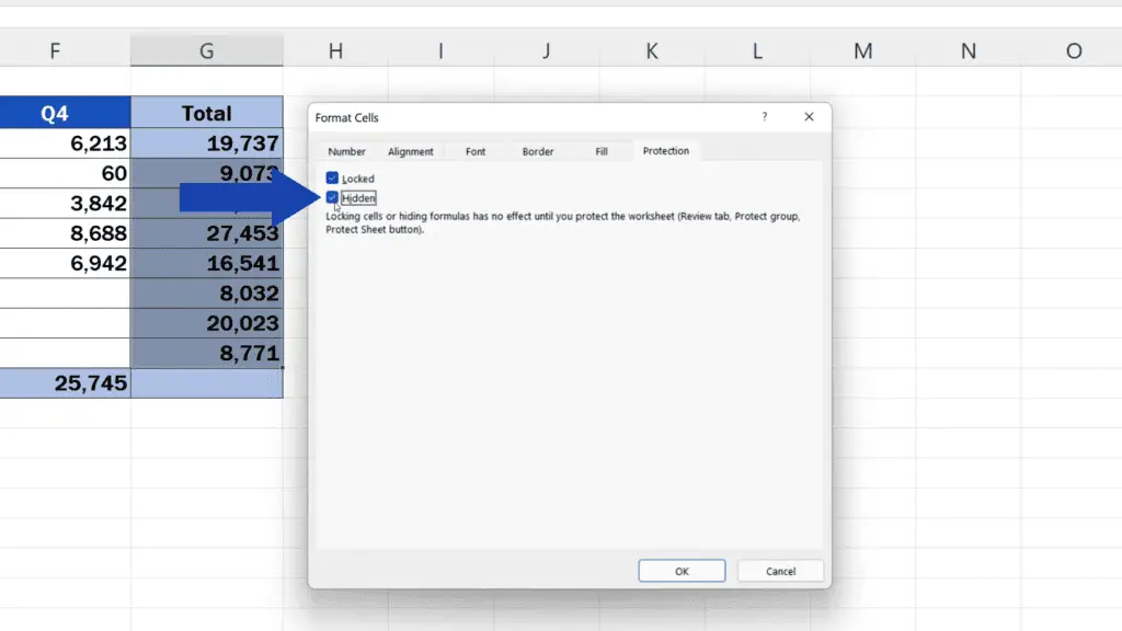
Confirm with OK and format the rest of the cells where you want to hide the formulas the same way. For example, we’re going to hide the sums here, in row 11, too.

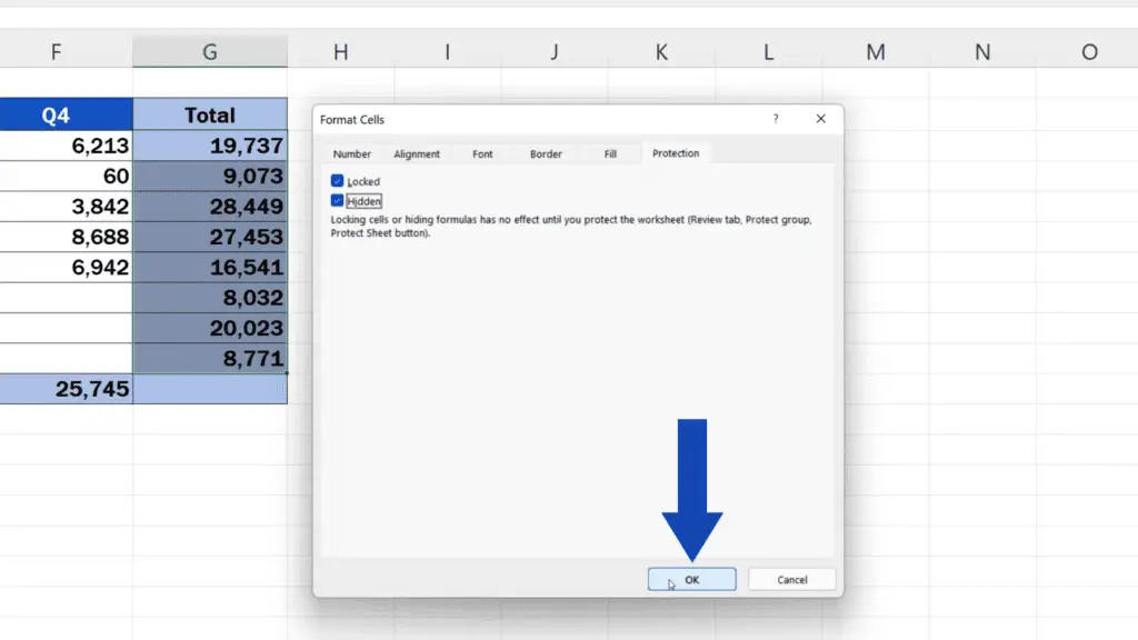
Now, you might notice that the cells have been formatted, but the formulas in them are still visible. This is because the Sheet must be protected first. You can do that through the option ‘Protect Sheet’ and we’ll go through this shortly.

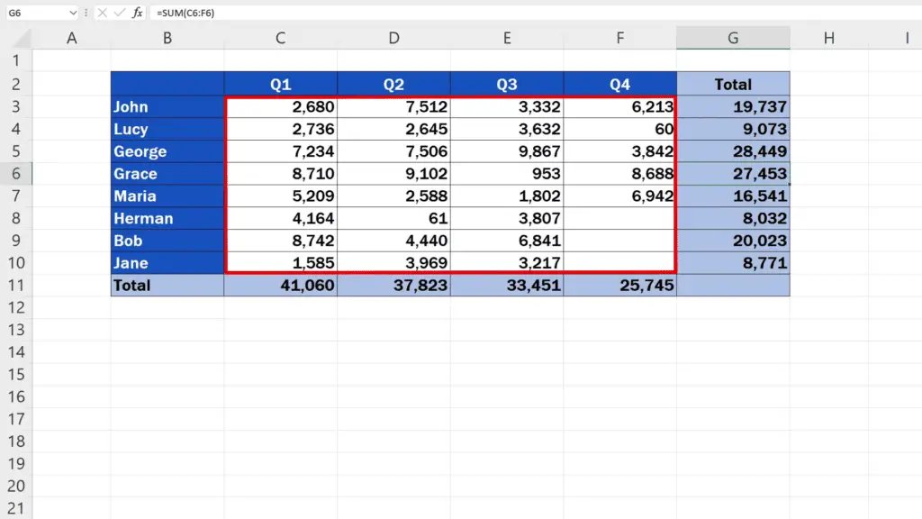
But before we do that, we need to identify the cells which should stay unprotected, which basically means we mark the cells which will stay editable and their contents will be accessible to everyone.

How to Protect Cells with Formulas

Let’s say we want our co-workers to be able to change the data in this table. To ensure that, we need to select the cells containing the data, right-click, select ‘Format Cells’ and in the tab ‘Protection’ unselect ‘Locked’.

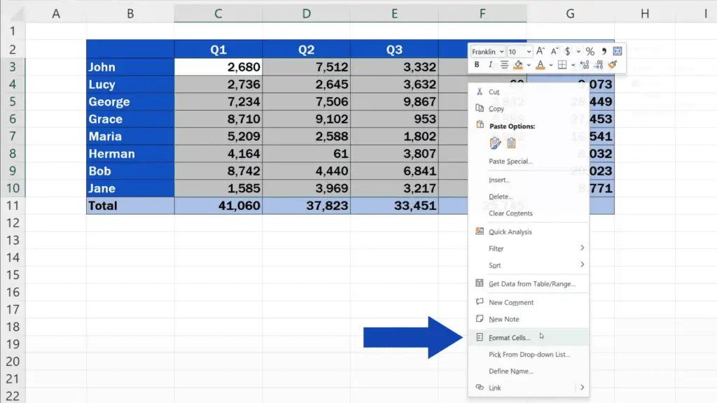
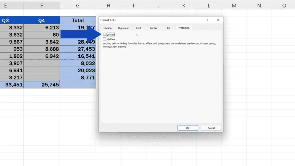
This way the cells will stay unlocked and anyone will be able to see and edit the information stored there. Now we click on OK and move on.

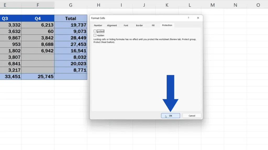
Once we’ve formatted all the cells as we needed and we’ve clearly marked the cells that should be locked as well as the ones that should stay editable, we can proceed with the last step.

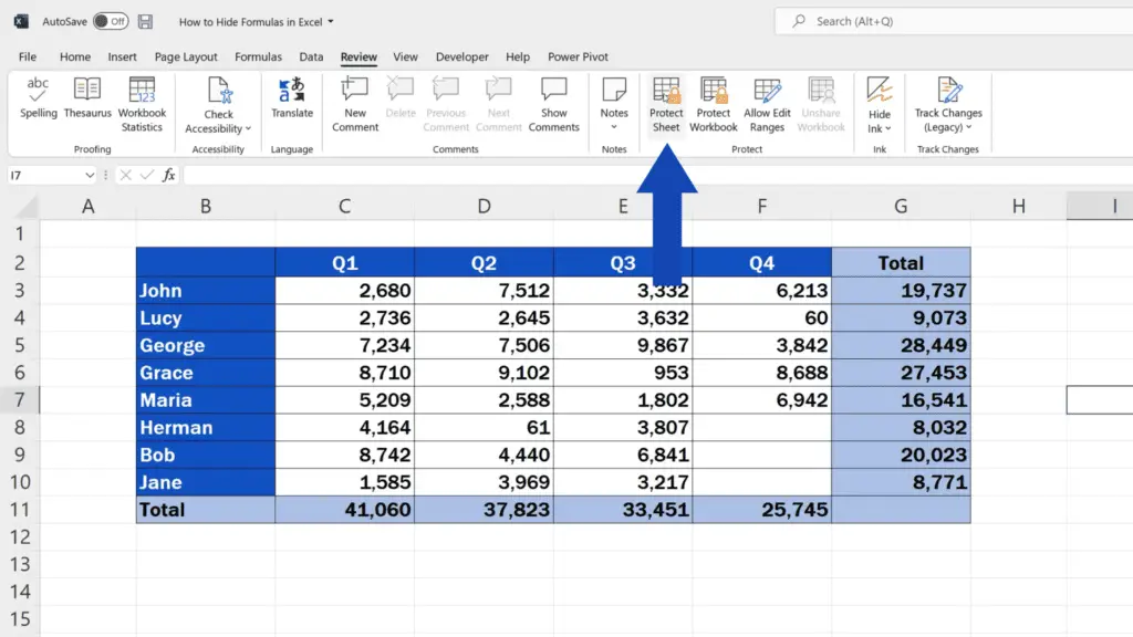
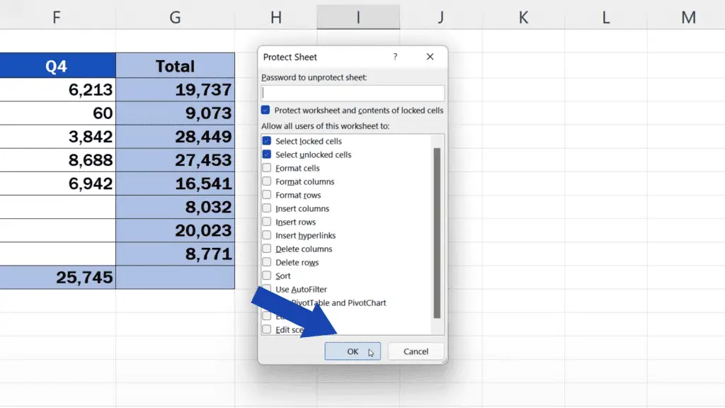
To put all of the settings in practice, we need to open the Review tab and click on the button ‘Protect Sheet’.

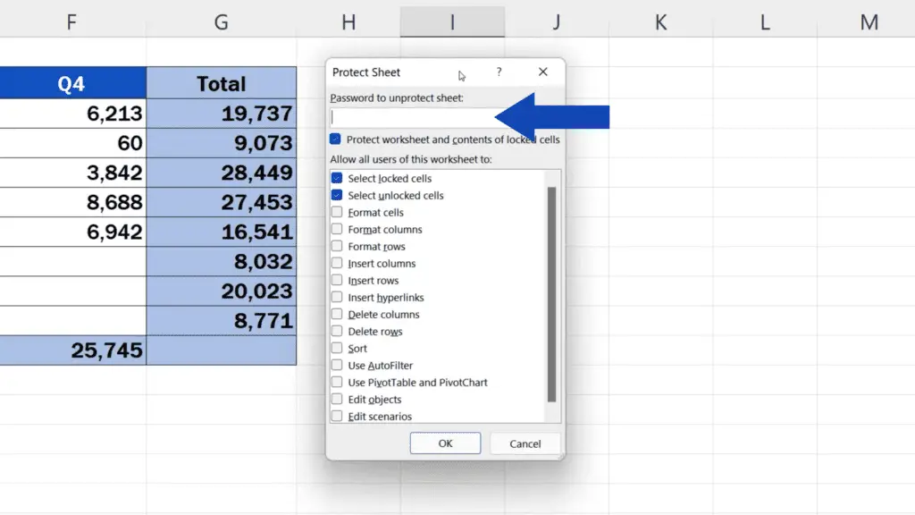
If needed, you can use a password to protect the sheet. We won’t use a password now, so we only confirm by clicking on OK and that’s it!

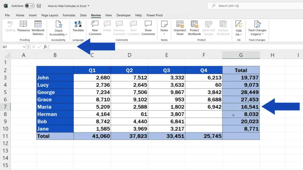
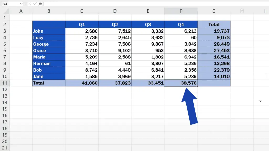
The formulas in the table are not visible, because they’ve been locked.

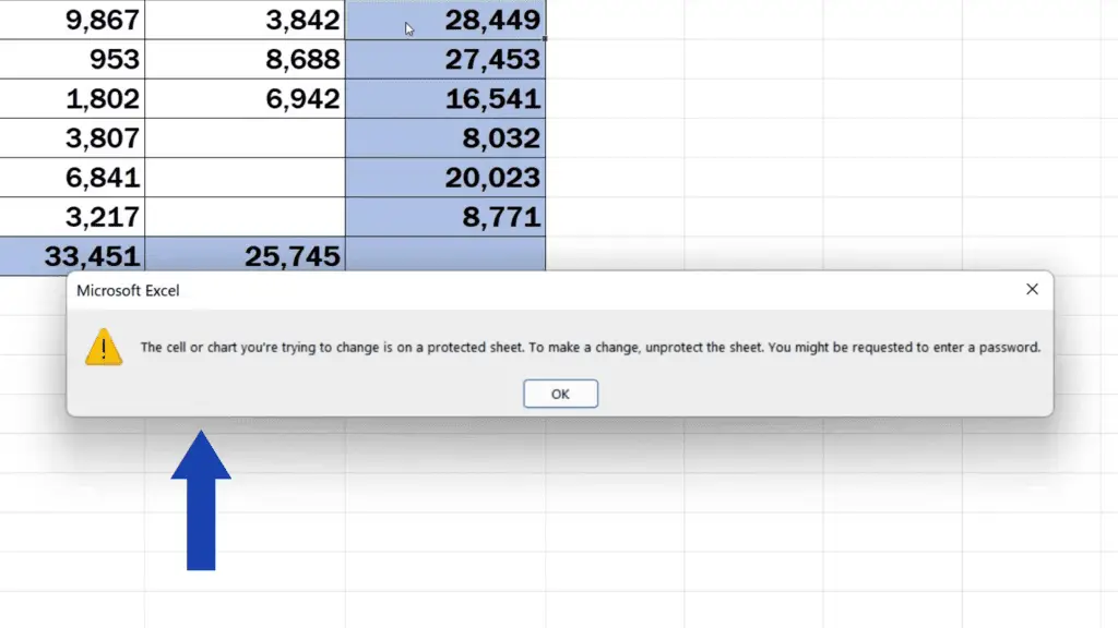
If someone would like to edit the locked cells, this message pops up.

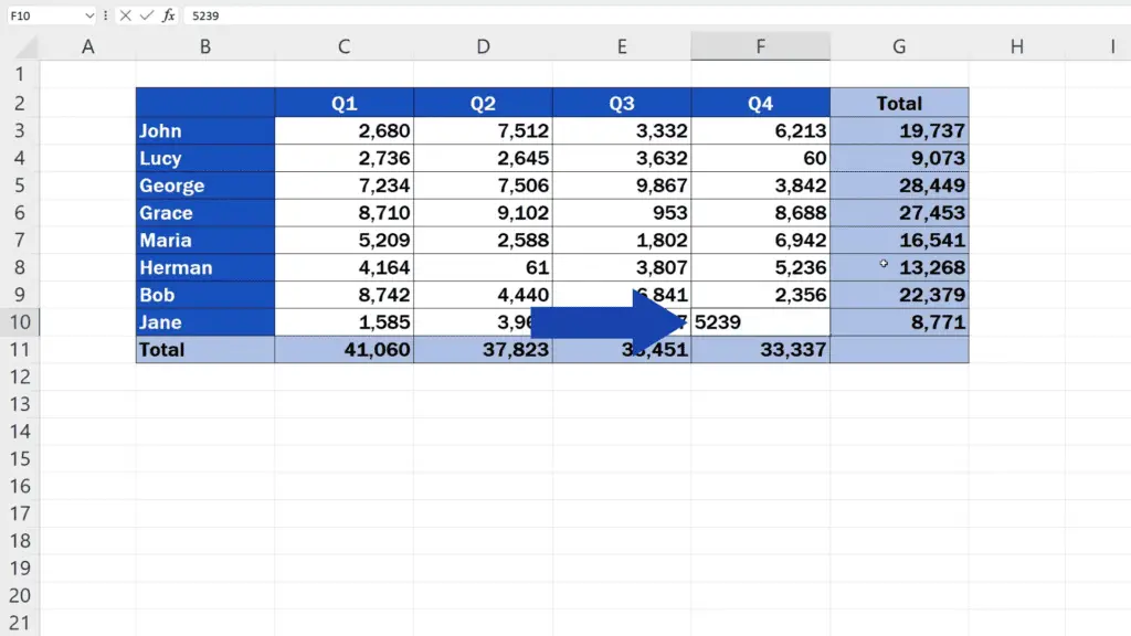
On the other hand, the cells storing the editable data can be accessed and the information inside them changed. And all the changes get reflected in the formula calculations.

How to Unprotect Cells with Formulas

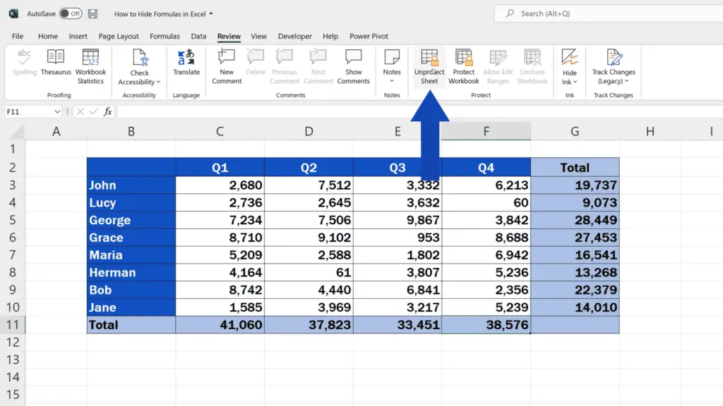
To turn the protection setting off, simply go to the Review tab and click on ‘Unprotect Sheet’. All the formulas are now visible and cells editable.

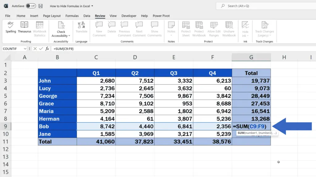
And if you’d like to know how to show formulas in Excel and how to be able to take a good look at all the formulas used in a spreadsheet, take a moment and watch the video tutorial the link to which has been provided in the list below.

Don’t miss out a great opportunity to learn:

• How to Show Formulas in Excel
• How to Protect Excel Sheet with Password
• How to Show or Hide the Formula Bar in Excel (Quick and Easy)

If you found this tutorial helpful, give us a like and watch other tutorials by EasyClick Academy. Learn how to use Excel in a quick and easy way!

Is this your first time on EasyClick? We’ll be more than happy to welcome you in our online community. Hit that Subscribe button and join the EasyClickers!

Thanks for watching and I’ll see you in the next tutorial!