How to Get Stock Prices in Excel (Free and Automated Solution)

In this tutorial, we’re going to have a look at how to get stock prices in Excel. Thanks to this solution, you’ll be able to access the most up-to-date information from stock exchanges all over the world.

Let’s get started!

Would you rather watch this tutorial? Click the play button below!

How to Fill in the Tickers

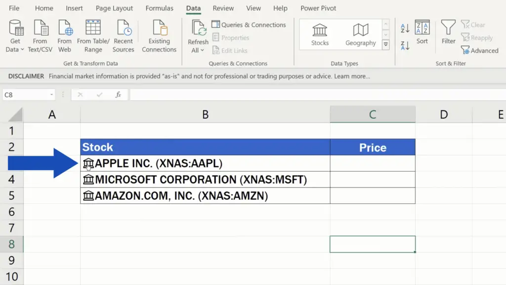
To begin collecting data from stock exchanges in Excel, first we need to fill in tickers or stock symbols for company names for which we want to get the information.

So here we’re going to fill in the tickers for the Apple, Microsoft and Amazon corporations.

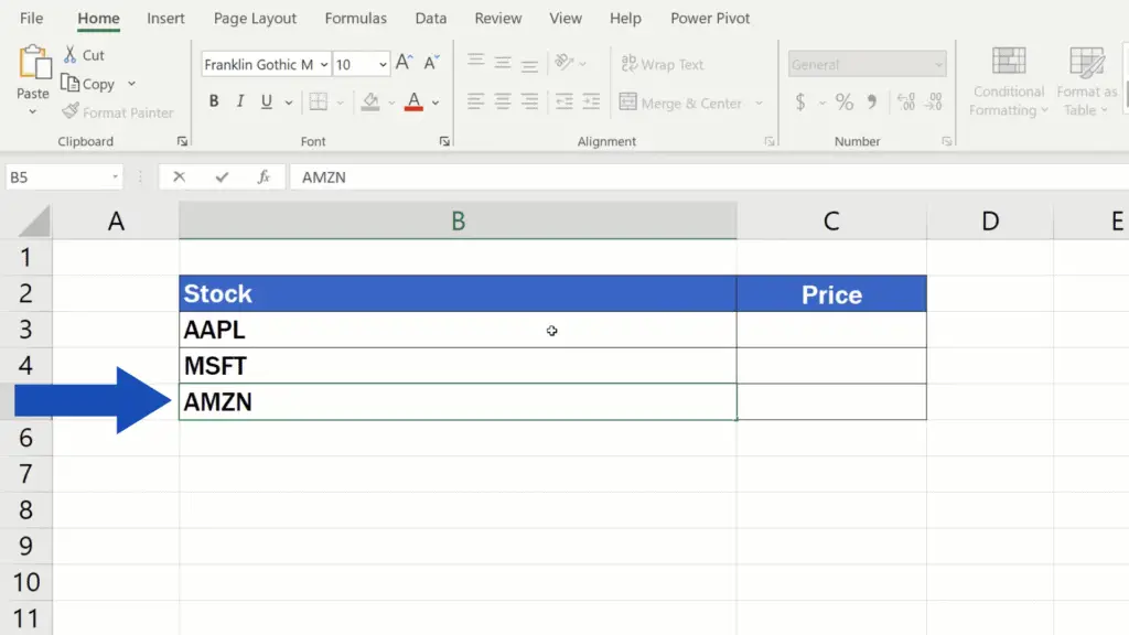
The use of tickers is recommended, because each ticker serves as a unique identifier of a company. Typing out companies’ names might seem more convenient but is imprecise and there’s a higher chance of introducing a typo in the data table, which would definitely affect the final result.

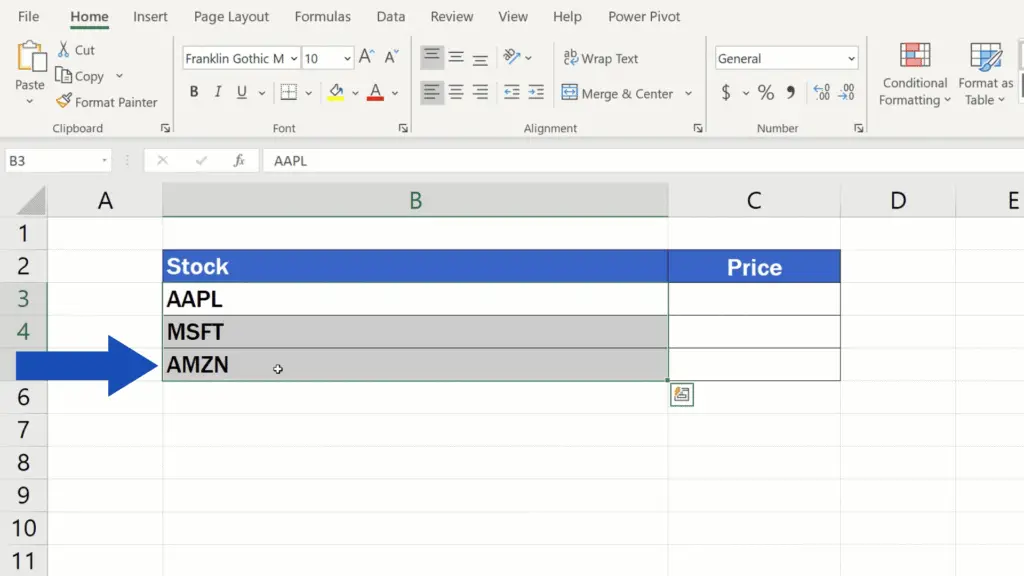
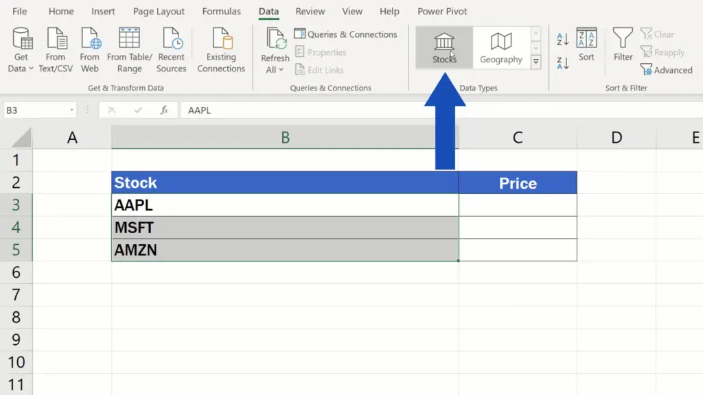
As soon as we’re done with filling in the tickers, we select the area that contains this information and click on Stocks in the Data tab.

Tickers get converted to a special data type where we can see the name of the company, the stock exchange from which we’ll be gathering information and the ticker of the company as used on that particular stock exchange.

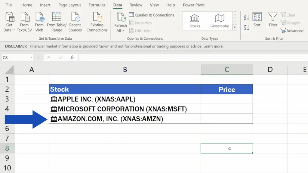
If we click on the Stocks icon located here, right before the information about the company name, we’ll see all available data that can be used in Excel.

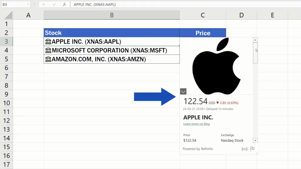
So, beside the price, there’s some more useful information.

It’s important to keep in mind though that this functionality which helps you access stock exchange information is available either in Excel 365 or the online version of Excel only. To get the latest Excel version, you can use the this link – https://www.easyclickacademy.com/buy-microsoft-office. By buying Excel, you’ll support EasyClick Academy and the tutorials it brings for you. Thank you!

How to Extract the Information on Stock Prices

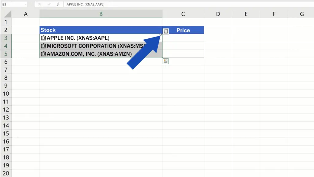
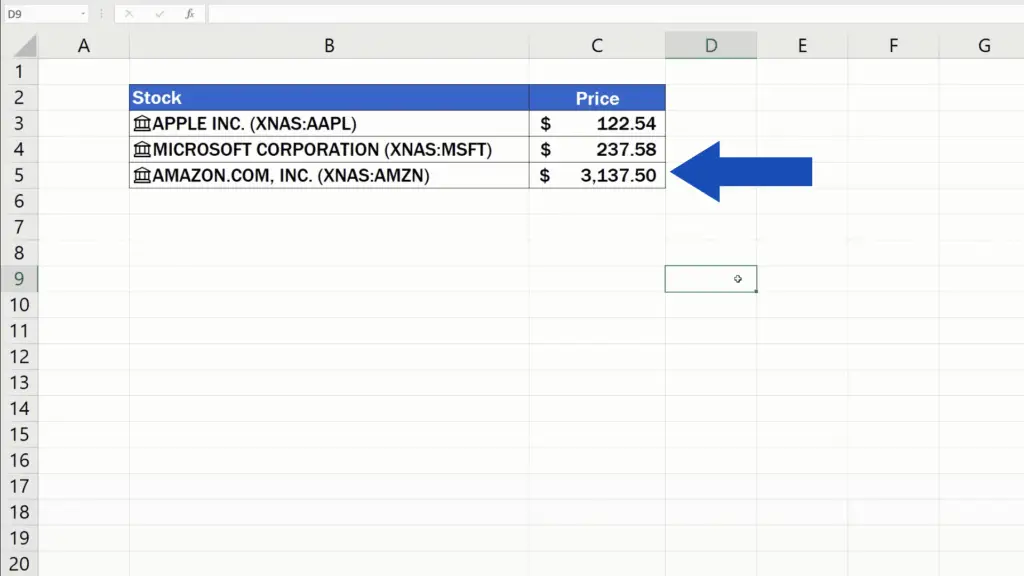
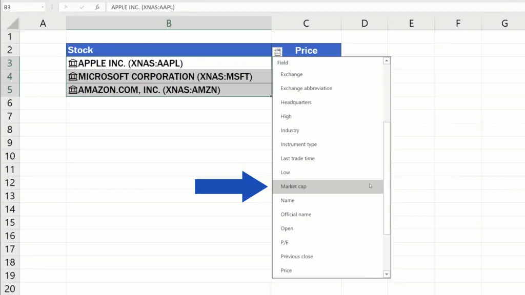
But let’s move on now and see how we can extract the information on stock prices in column C. Select the stocks and in the upper right corner we click on the icon for ‘Insert Data’. You’ll see a list of options from which you can choose the type of data you need. Since we want to get prices, we’ll click on ‘Price’ and here we go!

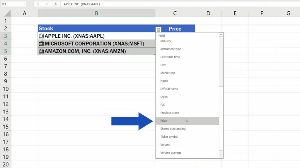
The current price for each stock now appears in column C.

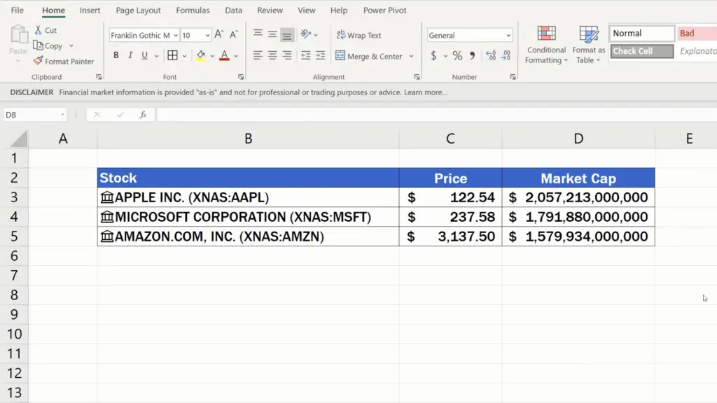
To use other data types, just open the list again and choose whichever necessary. Here, for example, we can add ‘Market Cap’, too, and tweak the formatting of the data table a little bit to make it look nice and neat.

How to Get Data from Another Stock Exchange

In case you want to get data from another stock exchange, right-click on the ticker, go to ‘Data Type’ and select ‘Change’.

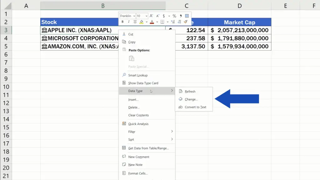
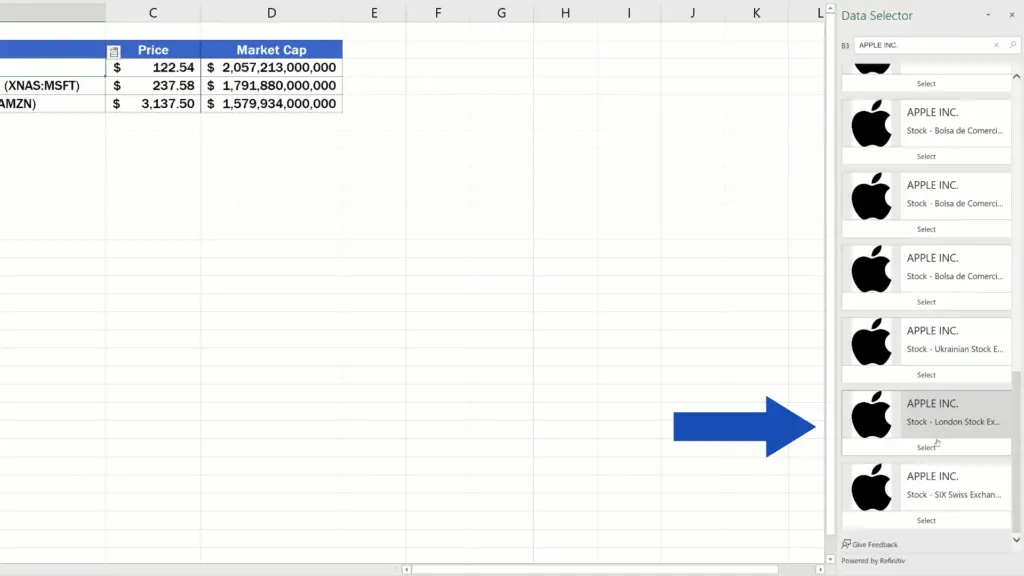
A pane appears on the right. Here we can delete the stock exchange identifier and the ticker, then we click on the Search icon and Excel shows the list of other stock exchanges.

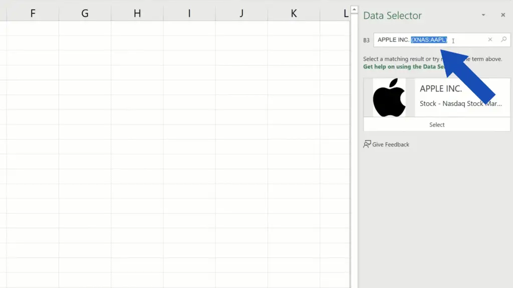
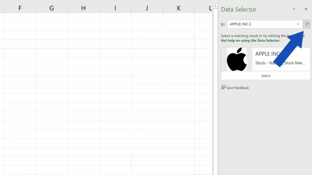
So, we can go for the London Stock Exchange, for example, and click on it to confirm the selection.

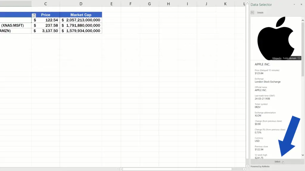
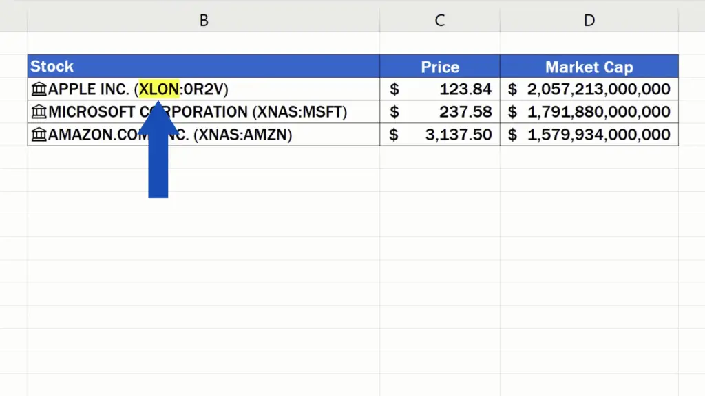
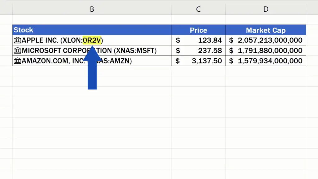
We can see that the information about the stock exchange for Apple has changed and the ticker has also changed according to the data used on the London Stock Exchange.

And that’s still not all we’re going to see today.

How to Get the Latest Information from the Stock Exchange

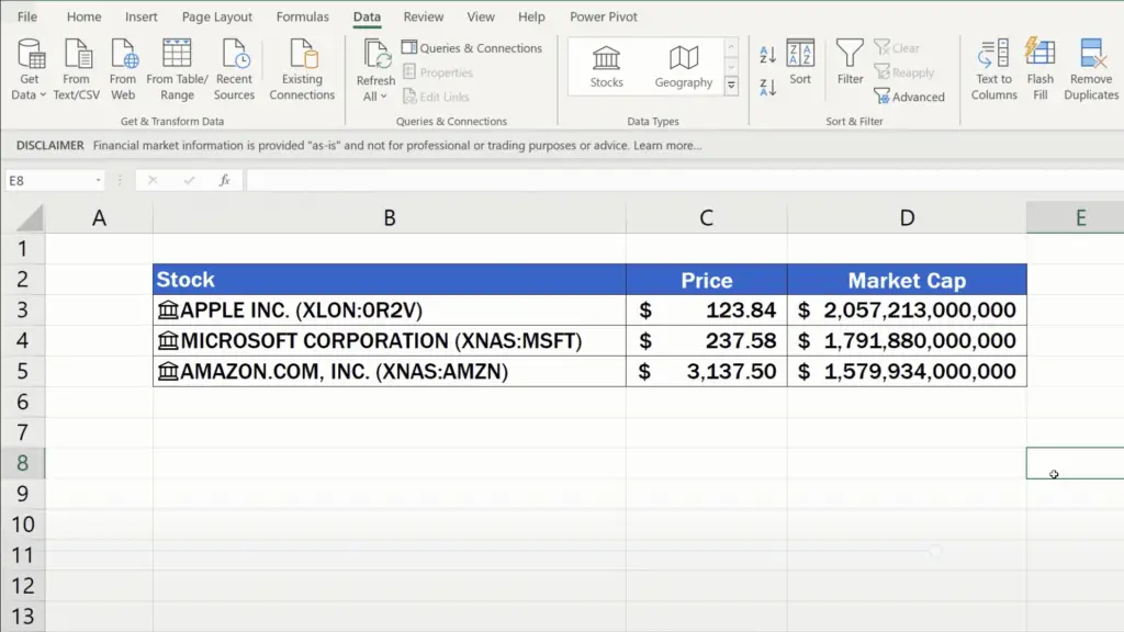
To get the most up-to-date information, we need Excel to refresh the data. So, go to the Data tab and click on the button ‘Refresh All’ and you’ll have the latest information from the stock exchange at hand.

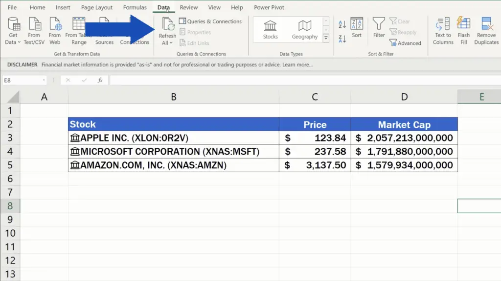
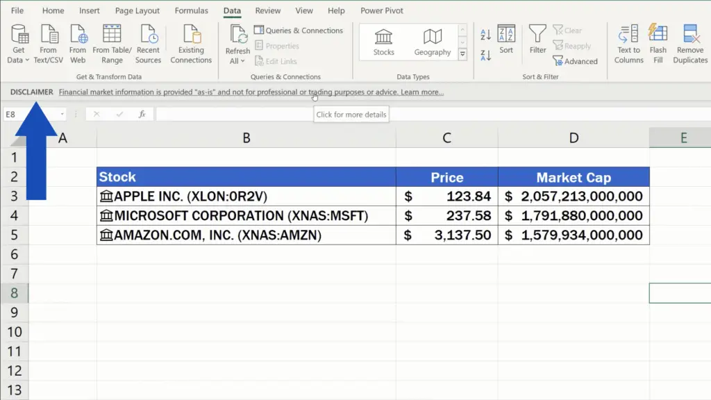
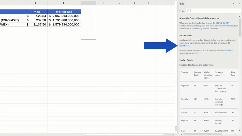
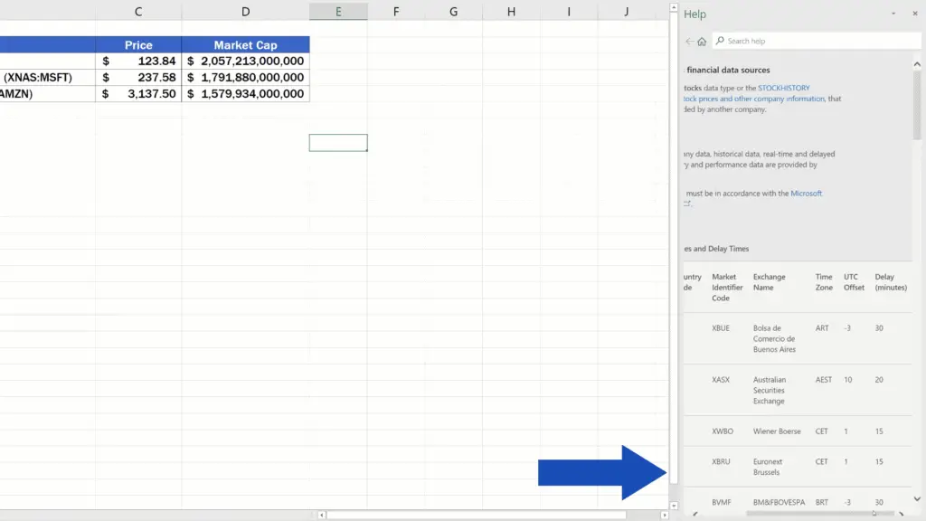
And before we wrap it up, it’s important to remember that the data from stock exchanges might come with a little delay. If you have a look here, there’s a disclaimer – click on it, you’ll see that the data are provided by the company Refinitiv and below you’ll find the information on Supported Exchanges and Delay Times.

Don’t miss out a great opportunity to learn:

• How to Calculate Percentage Increase in Excel (The Right Way)
• How to Calculate Age Using a Date of Birth in Excel (The Easy Way)
• How to Show or Hide the Formula Bar in Excel (Quick and Easy)

If you found this tutorial helpful, give us a like and watch other tutorials by EasyClick Academy. Learn how to use Excel in a quick and easy way!

Is this your first time on EasyClick? We’ll be more than happy to welcome you in our online community. Hit that Subscribe button and join the EasyClickers!

Thanks for watching and I’ll see you in the next tutorial!