How to Find Duplicates in Excel

In this tutorial, you’ll see a quick way how to find duplicate entries in an Excel table.

Let’s not waste any time – this is how to do it!

See video tutorial and transcription below:

See this video on YouTube:
https://www.youtube.com/watch?v=eAeFRAAwBe0

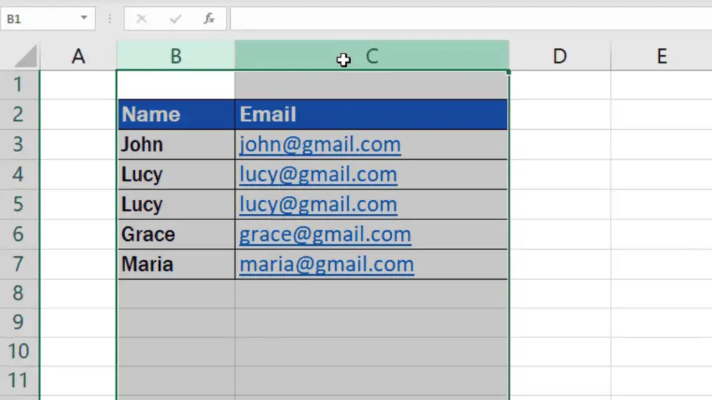
The first important step in finding duplicate data in a table is to define the area in which we want to look for duplicates.

Here we will select these two columns – columns B and C.

How to Highlight Unique Values in the Table

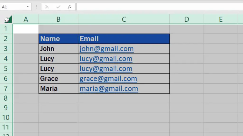
You can also highlight the whole sheet by clicking into the top left-hand corner if you wish to.

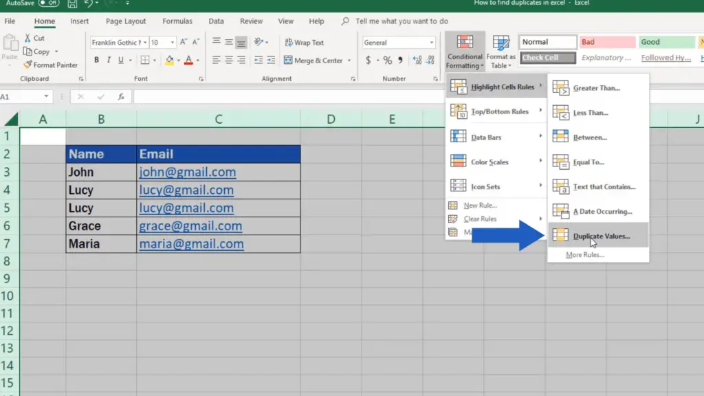
Go to the section Styles and choose Conditional Formatting option. Click on Highlight Cells Rules and select Duplicate Values.

Excel will immediately look for and highlights all duplicates in a table of any size. It doesn’t matter whether the table contains hundreds or thousands of entries.

In our table, we can see that duplicated data are located in rows 4 and 5.

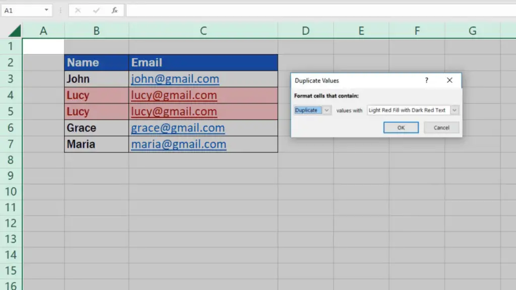
On the other hand, if we want to highlight unique values in the table, we would need to switch to ‘Unique’ in the drop-down menu.

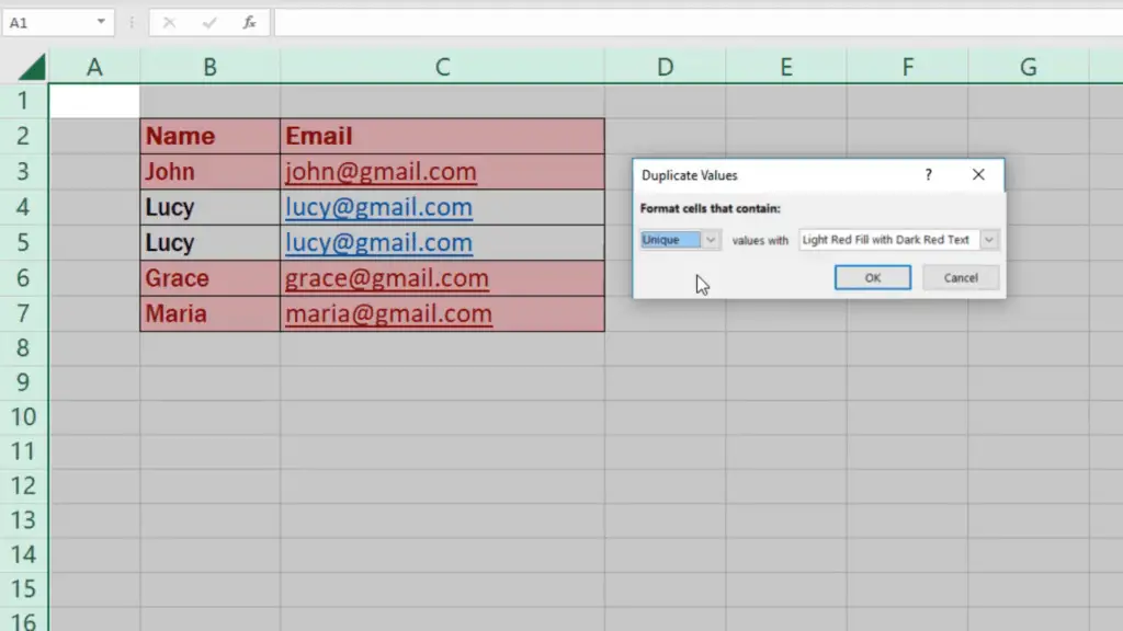
How to Change Colour Formatting of the Highlighted Data

Now, if we go back to the option ‘Duplicate’, we can change the color formatting of the highlighted data.

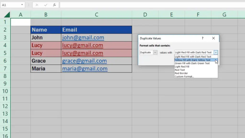
We confirm the choice by clicking on OK and the duplicates get highlighted within the table.

How to Turn Off the Highlighted Data

This highlighting of duplicates can be turned off by going back to the Styles section, clicking on Conditional Formatting again, and selecting Clear Rules.

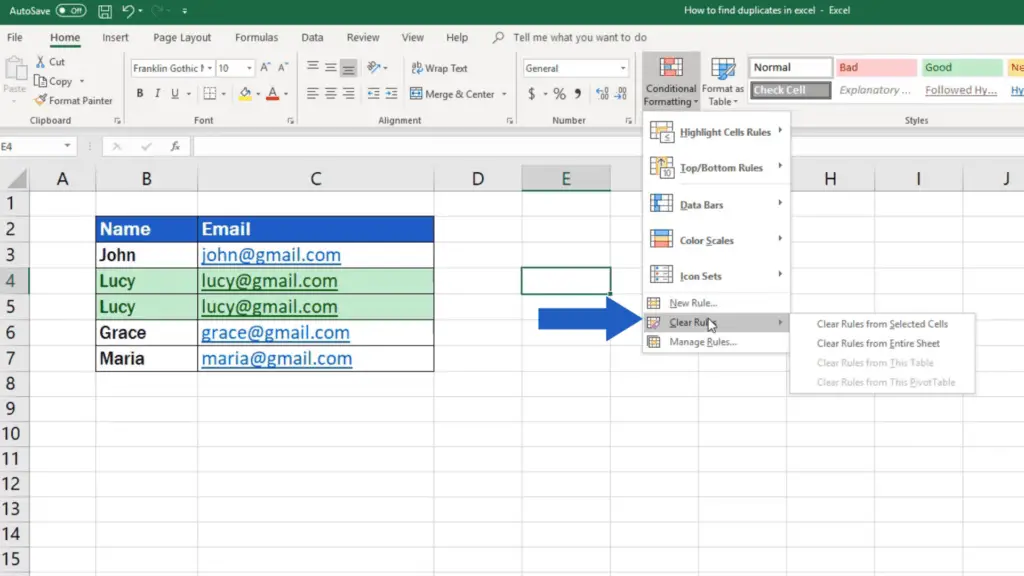
Here you can decide whether you’ll clear the rules from ‘Selected Cells’ only, or from the ‘Entire Sheet’. Let’s use the option ‘Clear Rules from Entire Sheet’, because we want to remove the formatting from the entire spreadsheet.

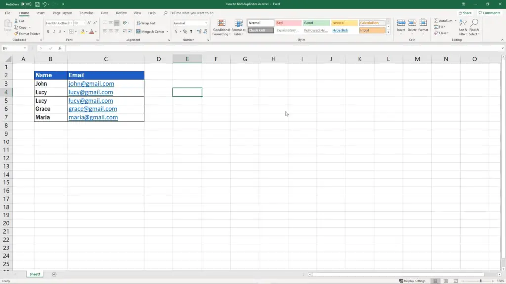
And we’re done! Highlighting of duplicates has been removed!

Don’t miss out a great opportunity to learn:

• How to Remove Duplicates in Excel
• How to Find the Largest Number in Excel
• How to Create a Drop-Down List in Excel

If you’ve found this tutorial helpful, like us and subscribe to receive more videos from EasyClick Academy. Look at more tutorials that help you use Excel quick and easy!

See you in the next tutorial!