How to Create a Hyperlink in Excel (3 Most Common Types of Hyperlinks)

In today’s tutorial, we’ll have a look at how to create a hyperlink in Excel. Thanks to hyperlinks, you’ll be able to access a specific file, web site or a place in the document in one click.

Let’s get started then!

Would you rather watch this tutorial? Click the play button below!

In Excel, we can create different types of hyperlinks and today we’ll have a closer look at the three most commonly used ones.

How to Create a Hyperlink to Existing File

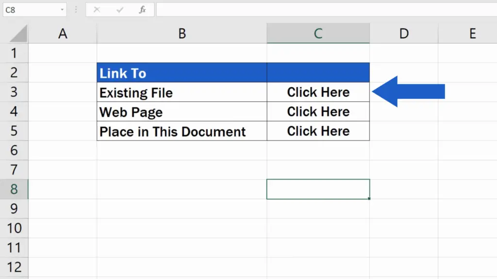
We’re gonna kick off with the hyperlink to an existing document, so to create the hyperlink, you’ll need to select a cell first, as usual.

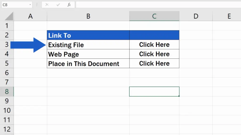
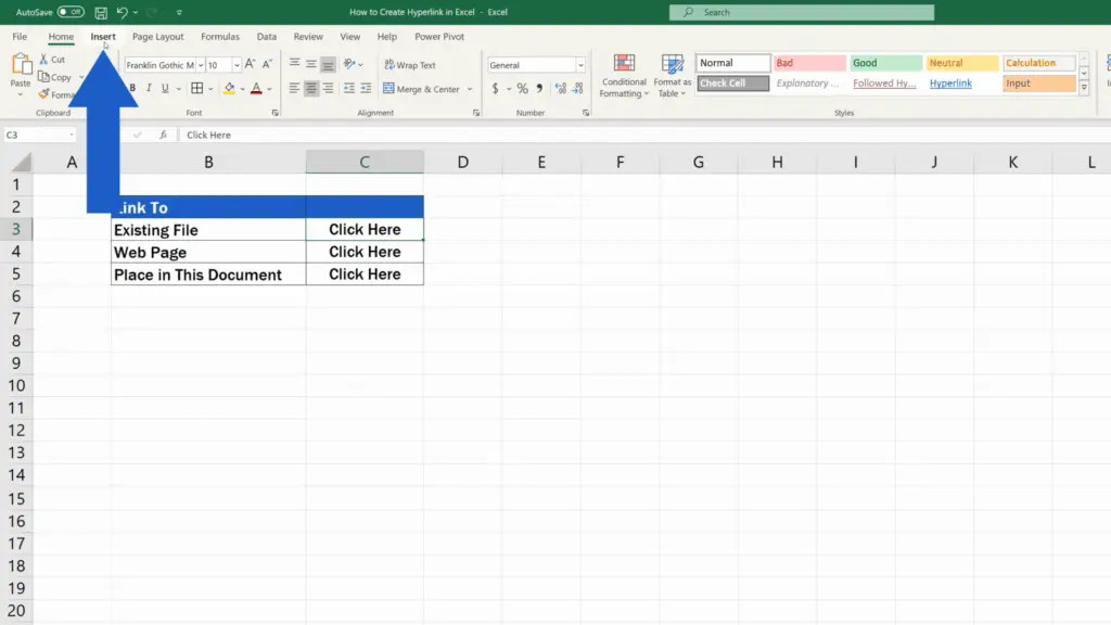
Let’s click on C3. Then we go to the Insert tab and select the option Link.

A pop-up window appears and you can choose where the inserted hyperlink will lead. The options are as follows:

• an existing file or a web page
• a place in the document
• you can create a new document with a hyperlink
• and an email address

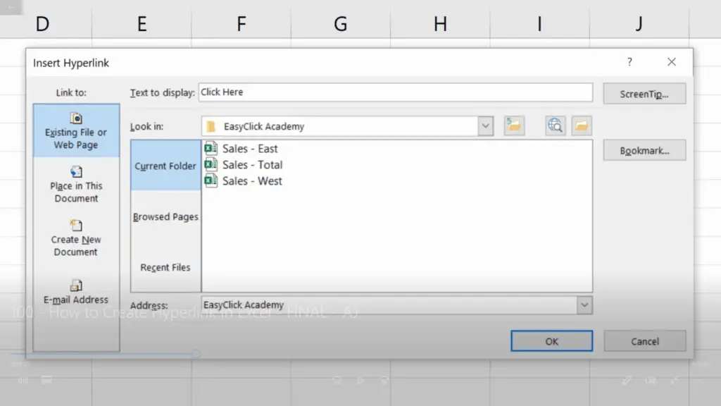
As we’ve already mentioned, today we’ll focus on the most commonly used options and we’re gonna go through them one by one.

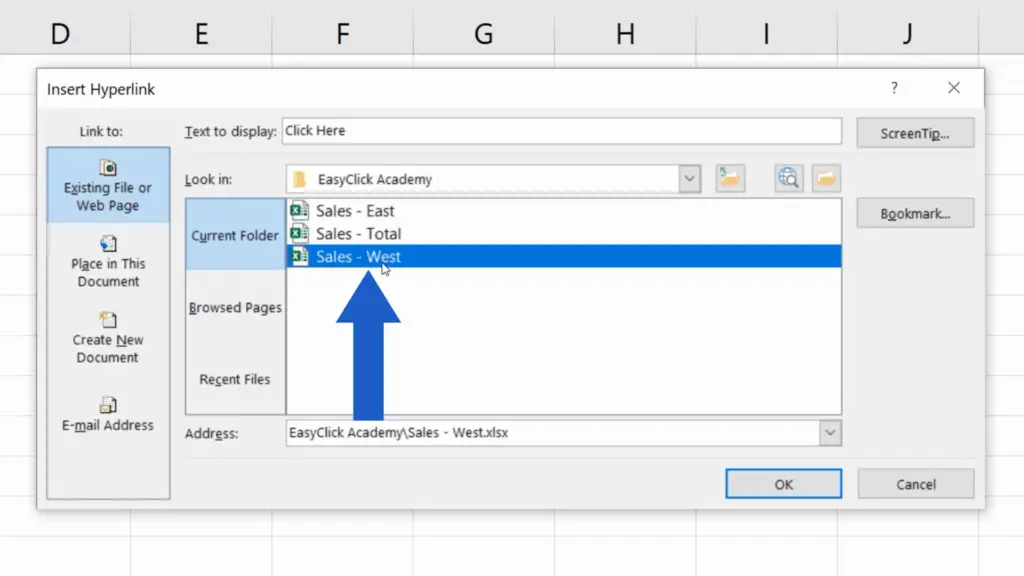
Since here, in the first example, we want to create a hyperlink which opens an existing document, we click on the first option – Existing File or Web Page and this is what we get.

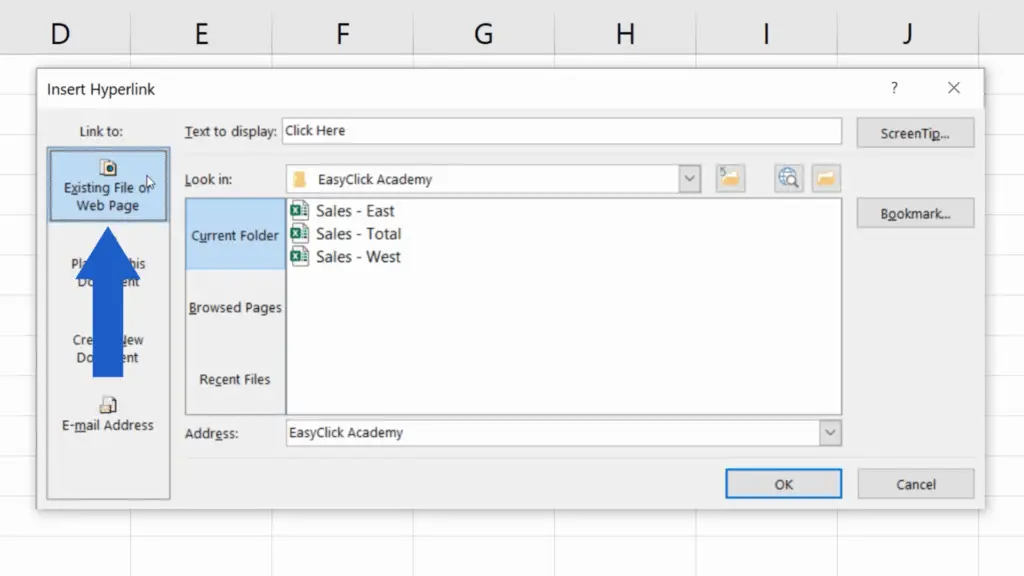
As you can see, here’s the folder ‘EasyClick Academy’ which contains three specific files.

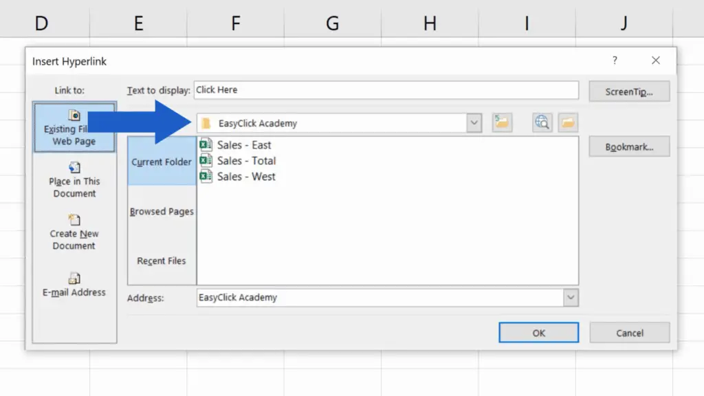
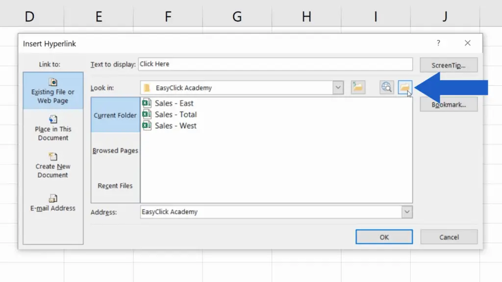
If you need to select a different file from another folder, you can use this option Browse to look for any file in your computer.

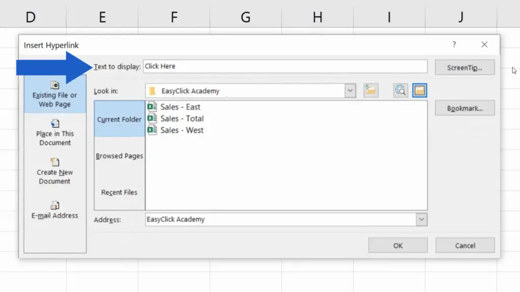
Each hyperlink comes with a text that displays in the cell. You can change the text according to what you need and you can do it here, in the field ‘Text to display‘. We’re gonna stick with ‘Click Here’ now and select the file ‘Sales-West’. Click on OK, and that’s the first hyperlink created!

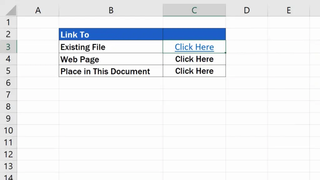
Let’s try it out.

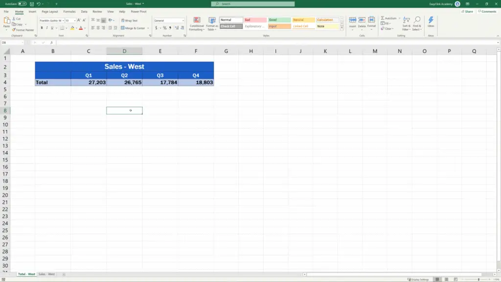
Click on the link and the file ‘Sales-West’ opens right away! Great! Now, close the file, we’ll carry on.

How to Create a Hyperlink to Web Page

The second most commonly used type of hyperlink is the one that takes you online, to a web page. Again, let’s click on the cell where we want to create the hyperlink, go to Insert, then Link.

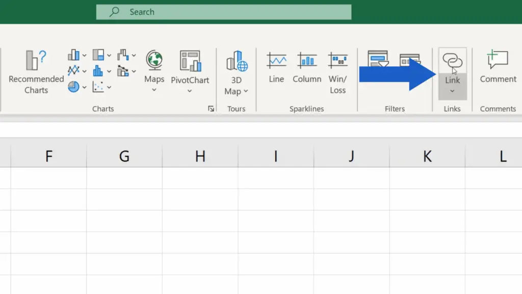
In the pop-up window you’re already familiar with, choose the option ‘Existing File or Web Page’ again. Now, down here, where you see ‘Address’, insert the URL address to which you want the hyperlink to lead.

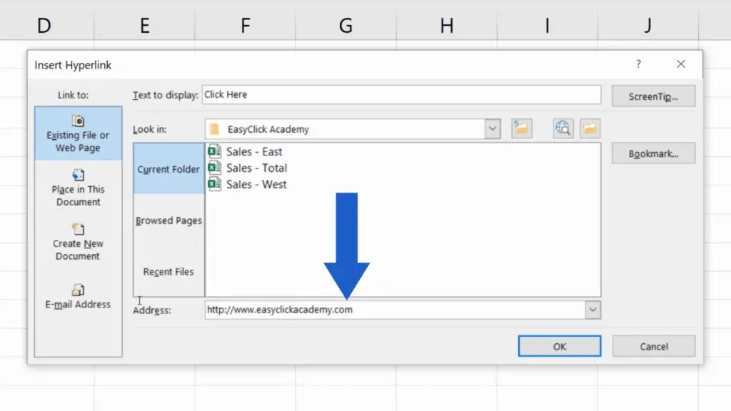
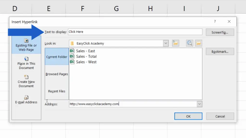
If you want to change the text to display with the hyperlink, you can do it up here. Again, we’ll leave it at ‘Click Here’ and hit OK.

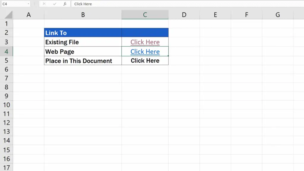
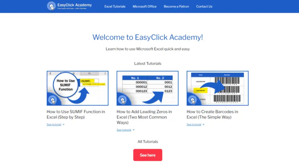
Ta-da! The second hyperlink’s here. When you click on it, it opens our web page, EasyClick Academy, which has been inserted here.

How to Create a Hyperlink to Place in the Current Document

And last but not least, let’s have a look at how we can create a hyperlink leading to any place in this document.

The first steps are practically the same as in the previous two cases. Click on the cell and select Link. But instead of the first option, go for the second one – ‘Place in This Document’.

Excel now lists the sheets in this document. There are two sheets here, so we’ll pick the second one – Sales – to create the hyperlink leading there.

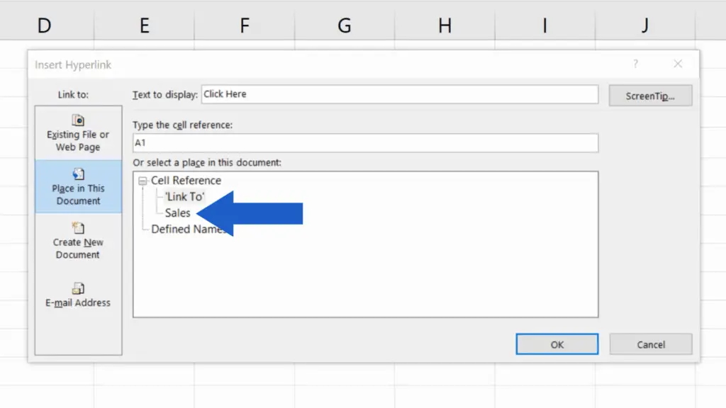
Select the sheet and if you want the cursor to land on a specific cell within the sheet, you can enter the cell reference in the field ‘Type the cell reference’.

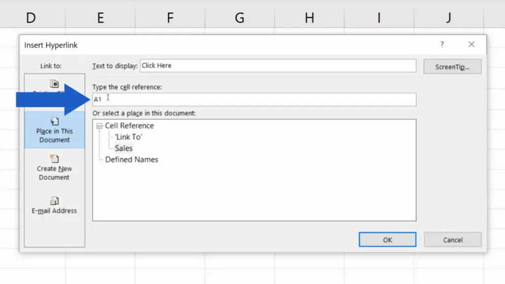
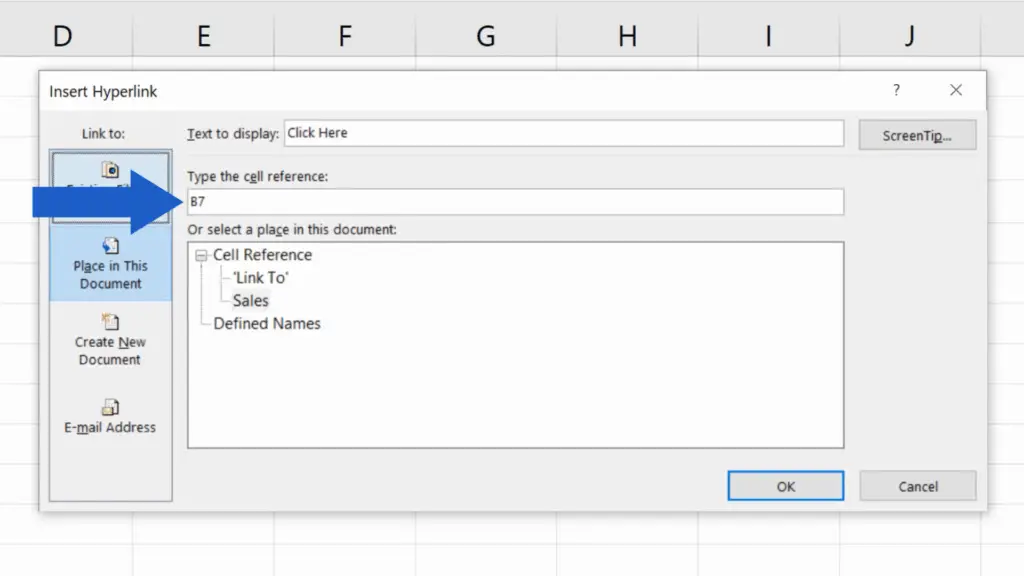
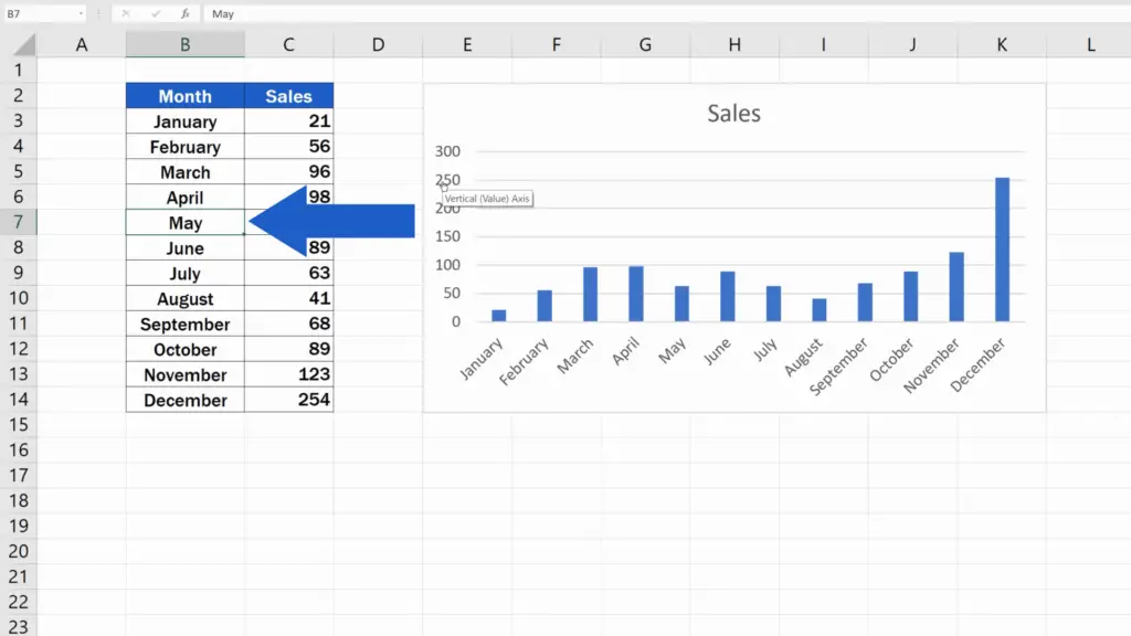
Currently it displays the coordinates A1. Let’s change that to let’s say B7 and click on OK.

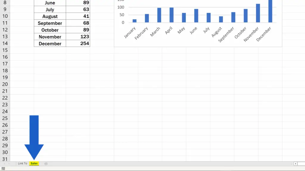
If you now click on the link, Excel will open the sheet with sales which we selected a while ago in the pop-up window and the cursor has been set on the cell B7.

The same way works if you need to create a hyperlink to an email address or create a whole new document. In the pop-up window ‘Insert Hyperlink’ simply select the right option.

And if you’re by any chance wondering how to remove these links, watch our tutorial on how to remove hyperlinks in Excel. The link to this tutorial is in the below below.

Don’t miss out a great opportunity to learn:

• How to Remove Hyperlinks in Excel
• How to Rename Sheet in Excel
• How to Hide Sheets in Excel

If you found this tutorial helpful, give us a like and watch other tutorials by EasyClick Academy. Learn how to use Excel in a quick and easy way!

Is this your first time on EasyClick? We’ll be more than happy to welcome you in our online community. Hit that Subscribe button and join the EasyClickers!

Thanks for watching and I’ll see you in the next tutorial!