How to Count Unique Values in Excel (Quick and Easy)

Today we’re going to have a look at how to count unique values in Excel. We’ll be talking about two different senses of the word ‘unique’, hence two different ways to count unique values, both quick and easy. That way, you’ll be able to pick the right calculation depending on the situation.

Let’s start!

The word ‘unique’ can be understood in two ways and that’s why we’re going to talk about two kinds of unique values and two ways you might want to count them in Excel.

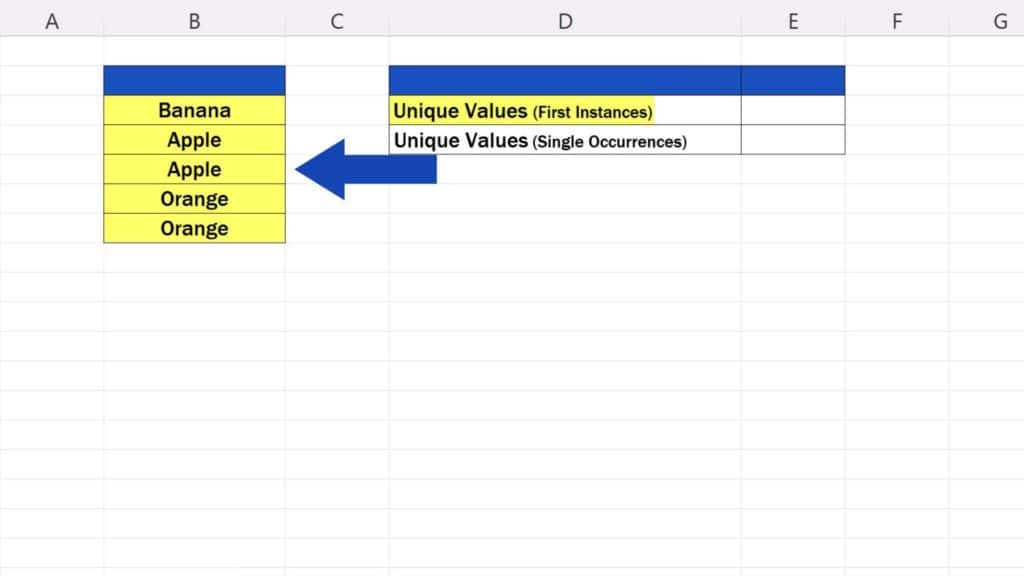
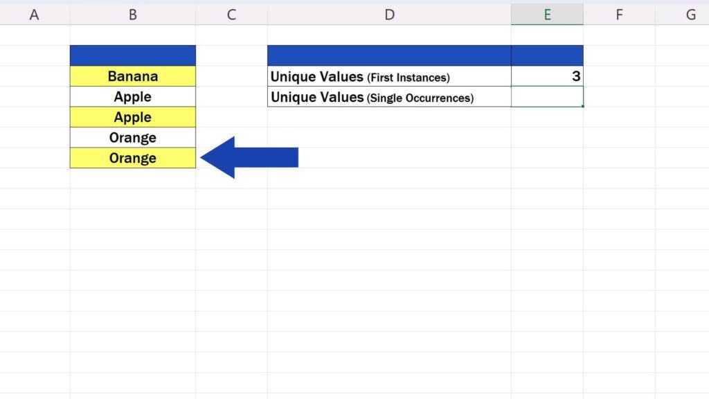
1. The first kind of unique values is when we’re talking about ‘unique’ in the sense of the first instance of a value. That means that in a data table, these unique values may occur only once or they may have duplicates. For example, here are three unique values and these are: ‘banana’, ‘apple’ and ‘orange’. The whole table contains three unique values, but some of these values are duplicated. ‘Apple’ and ‘orange’ occur in the table twice, ‘banana’ only once.

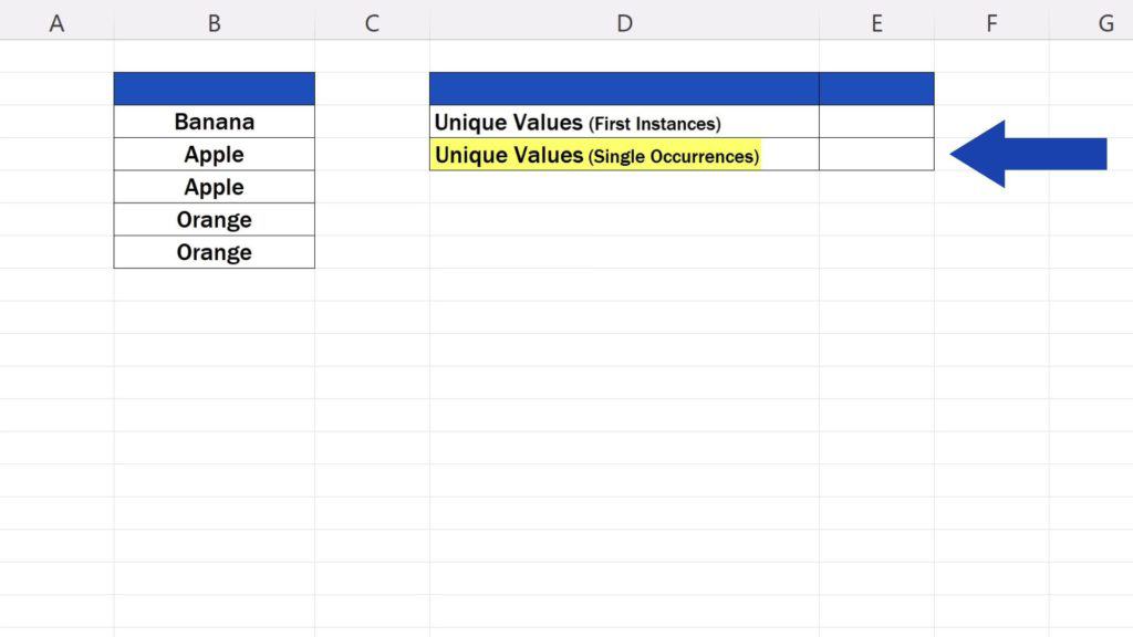
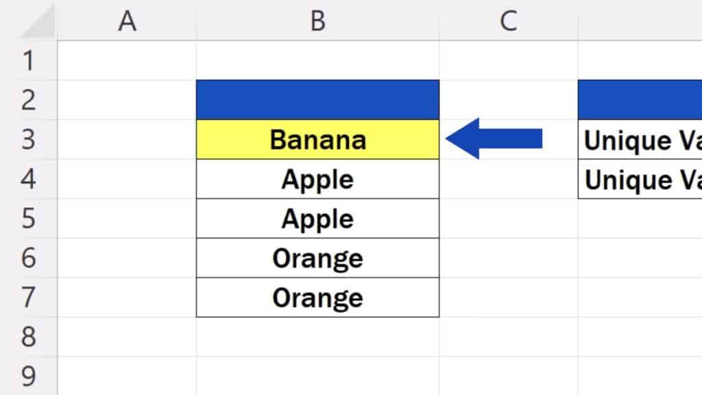
2. The other kind of unique values is in the sense of ‘single-occurrence’ values. In this calculation, we want to count the values that occur in the data table only once, which means that the values that have duplicates won’t be included in the count at all. In our case, there’s only one value like that: ‘banana’. It’s the only value with a single occurrence, without duplications.

So, let’s see what formulas there are to count both kinds of unique values.

First, we’ve got to state that there’s no simple way to count unique values. We’ll be using quite complicated formulas to do this. However, there are various ways to come up with a unique value count and here’s one of the easiest ones.

The good news is that you don’t need to understand the formulas in their essence. You can simply copy them from the list below and modify them according to your needs.

• Unique Values (Among Duplicates)
  =SUMPRODUCT(1/COUNTIF(***,***))
  
• Unique Values (Without Any Duplications)
  =SUM(IF(COUNTIF(***,***)=1,1,0))

Here’s how.

How to Count Unique Values in Excel – First Instance

Let’s start with the unique values as first-instance values.

Copy the first formula and paste it in the target cell. Highlight the first set of asterisks and enter the range of the data in which you’d like to count unique values instead.

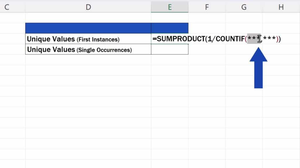
In this data table, it’s the cell range B3 to B7. Then enter the same range once again, right behind the comma, by replacing the second set of asterisks.

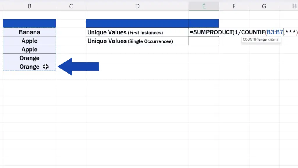
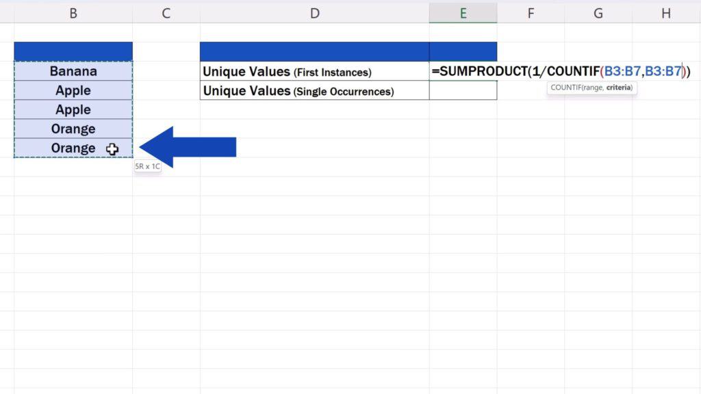
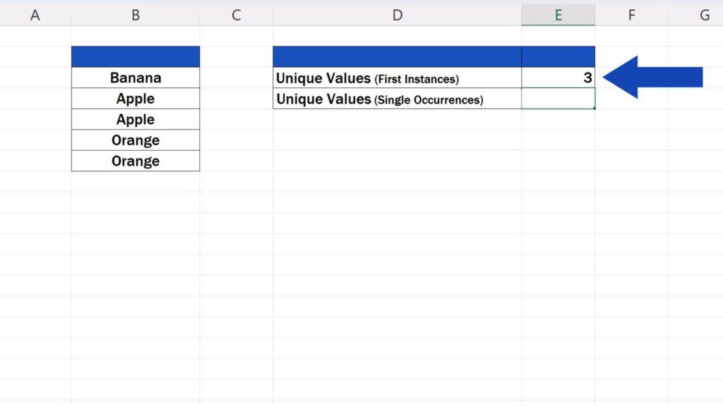
Once done, press Enter and here we go with the result! As we’ve already mentioned, these unique values count all first instances of the values, including the values that have duplicates. Here we’ve got three unique values: ‘banana’, ‘apple’ and ‘orange’.

Of course, if you’d like to understand the formula in detail, we can have a look at that, too. Just leave us a note in the comments section and we can make a separate video tutorial about that. But now we’re not going to dig deep into what these formulas mean and contain. Our aim is to see how we can work with them and use them in practice or to discuss what problems you might encounter while trying to use them.

Before we move on, let’s try the other formula. The one which counts all unique values as single-occurrence values in a data table, which is the values without any duplications.

How to Count Unique Values in Excel – Single Occurrences

Again, this formula is in the above, so just copy it into the target cell and use the sets of asterisks as a placeholder for the correct cell range.

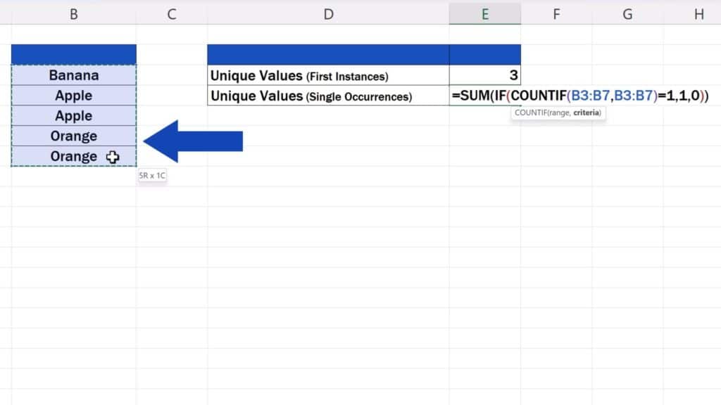
And that’s it! There’s only one unique value with a single occurrence in our data table, and that is ‘banana’.

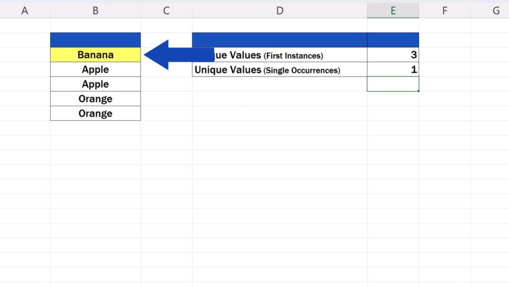
So, let’s fiddle with both calculations a bit and replace the value ‘apple’ in B4 with ‘lemon’. Have a look at the result – now we’ve got four unique (first-instance) values that can have duplicates and three unique (single-occurrence) values with no duplicates.

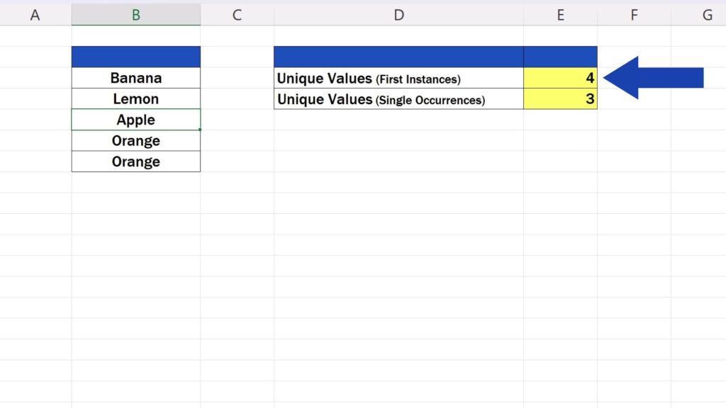
These formulas work with number values, too. So, if we change the text ‘orange’ in B6 to number 1, Excel will update the results again.

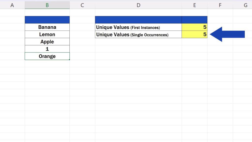
Of course, there’s a little complication you may encounter.

How to Count Unique Values in Excel with Empty Cells

If we delete data, for example we remove the value in the cell B5 and the cell stays empty, the first formula will show error. That’s why it’s important to remove all empty cells from the data table before we use the formula. You can have a look at how to do that in a tutorial on how to remove blank rows in Excel.

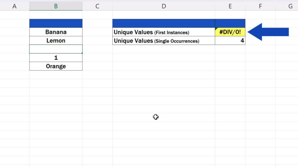
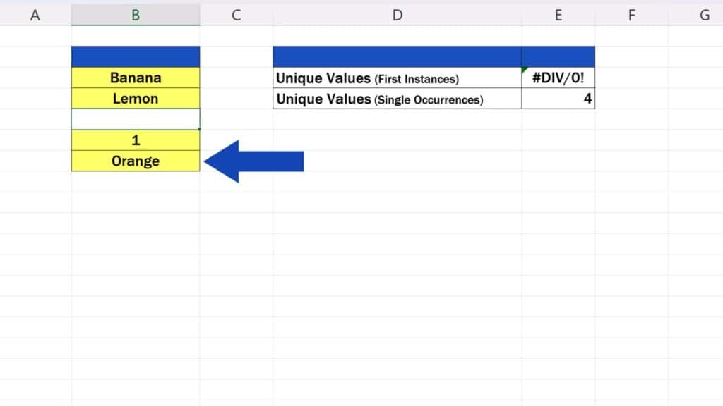
The second formula works fine with empty cells. It takes into account only the cells that contain data. That’s why the result shows four, as there are four unique values without duplicates in our data table.

Do you already know which of the two formulas you’ll be using more often? Leave us a comment in the comments section below. We’ll be happy to hear from you!

Don’t miss out a great opportunity to learn:

• How to Remove Blank Rows in Excel – BASIC
• How to Remove Blank Rows in Excel – ADVANCED
• How to Highlight Blank Cells in Excel (Conditional Formatting)

If you found this tutorial helpful, give us a like and watch other tutorials by EasyClick Academy. Learn how to use Excel in a quick and easy way!

Is this your first time on EasyClick? We’ll be more than happy to welcome you in our online community. Hit that Subscribe button and join the EasyClickers!

Thanks for watching and I’ll see you in the next tutorial!