How to Copy and Paste Formulas in Excel without Changing Cell References (Quick and Easy)

In this video tutorial, we’re going to see how to copy and paste formulas in Excel without changing cell references. First, we’ll be talking about how to simply copy and paste a single formula without changing cell references and then we’ll move to a whole range of cells containing a formula and see how it works there.

Shall we start?

How to Copy a Formula Without Changing Cell Reference

To copy and paste a formula contained in one cell without changing cell references, we can’t simply copy the cell itself and paste it wherever we need. If we do that, the cell references within the formula change.

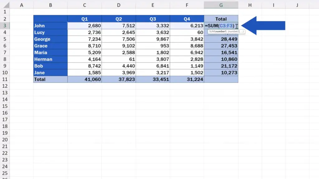
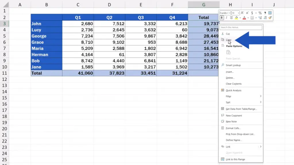
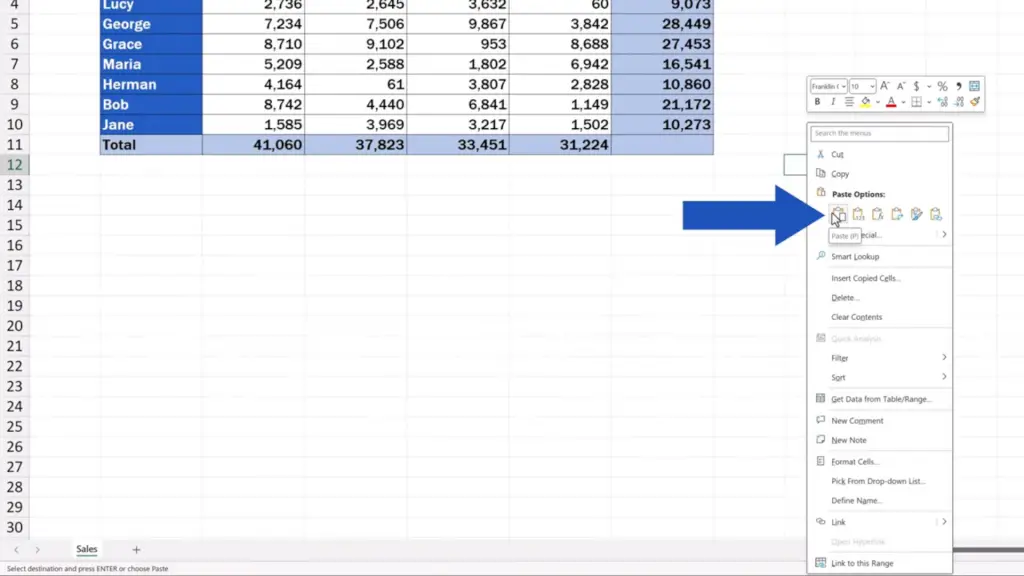
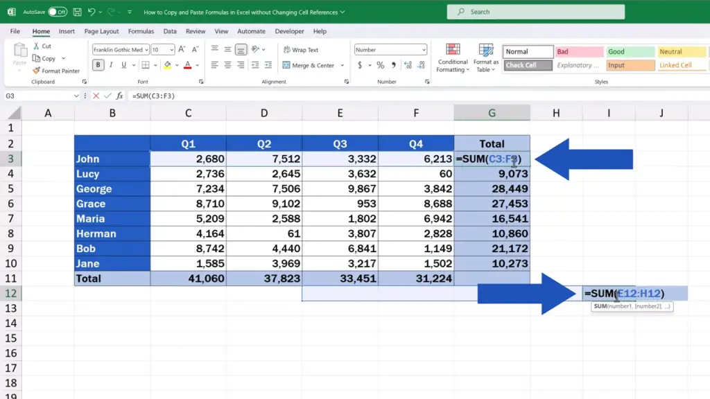
There are situations, though, where this can come handy and we can go through these in another video tutorial. However, if we don’t want the cell references to change, we need to work differently.

Let’s undo the last changes and have a look at how to copy one cell without changing the cell references in the formula it contains. Of course, there are more ways to do that, but here we’ll cover the one which is, in our opinion, the simplest and most useful way.

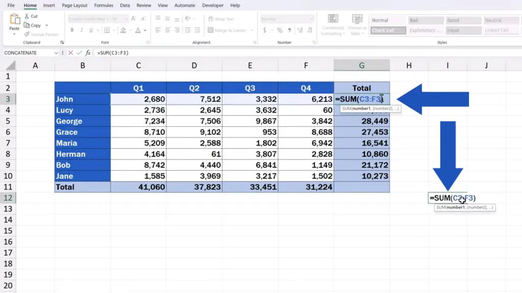
First, click on the selected cell. Now, click into the formula bar up here and copy the text of the formula using the Control and C keys.

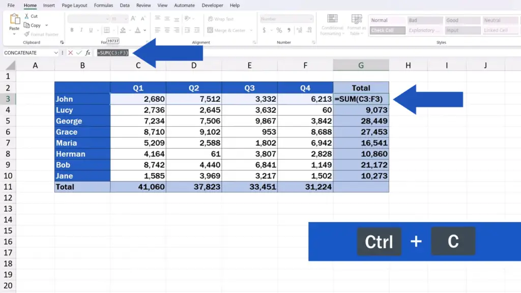
Press Escape to get out of the cell.

Once the text of the formula’s been copied, click into a target cell. Our target cell will be I12, so we click into this cell. Now, we click into the formula bar again and paste the copied formula. We can do so using the hot keys Control + V.

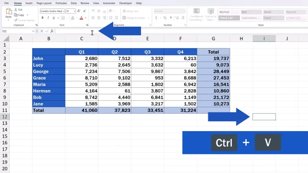
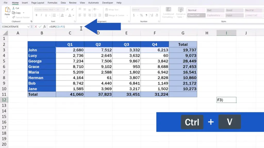
We hit Enter and here comes the formula inserted in I12 with no cell references changed.

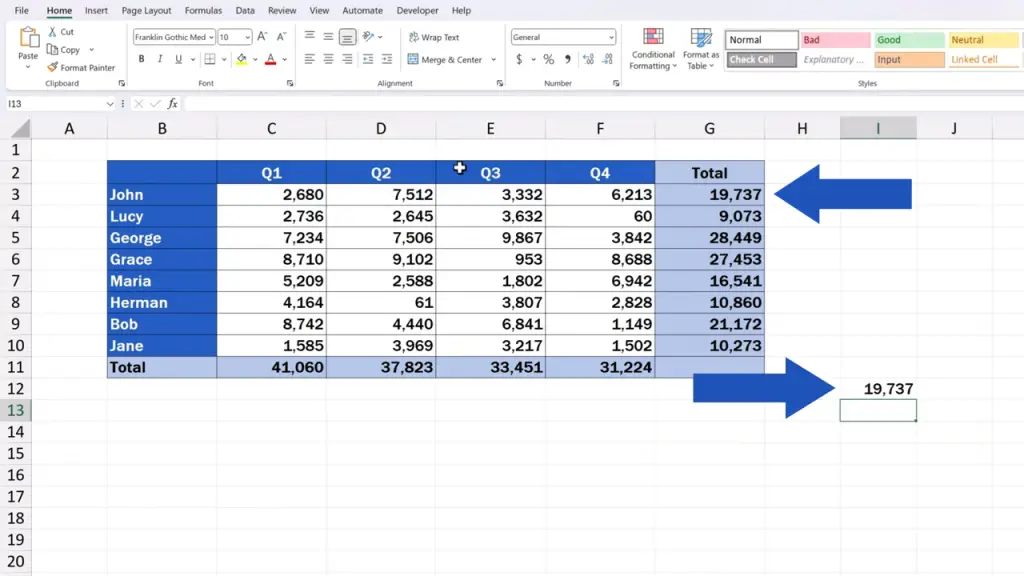
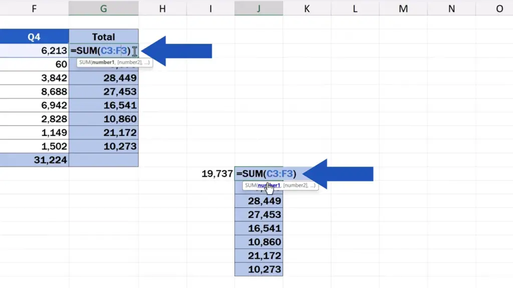
Once we press Enter again, we’ll see that both cells I12 and G3 contain the same formula with the same cell references, which basically means that both cells show the sum of the cell range from C3 to F3.

And let’s move on now.

How to Copy a Range of Formulas Without Changing Cell References

Let’s have a look at how to copy and paste a whole range of cells containing a formula without changing cell references.

Again, there’s a number of ways to do that in Excel. Here, we’ll be talking about the way which is, in our opinion, the most convenient and practical.

If we simply select and copy the cells in column G and paste them here in column J, the cell references change.

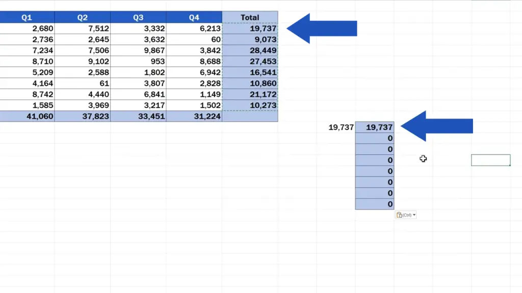
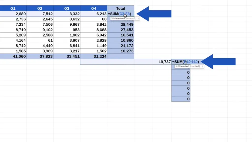
Let’s undo the changes again and take a look at how to copy the formula in the cells without changing cell references.

First, select the range of the cells containing the formula we want to copy. We’ll select all the cells containing the formula in column G. Then go to the ‘Home’ tab.

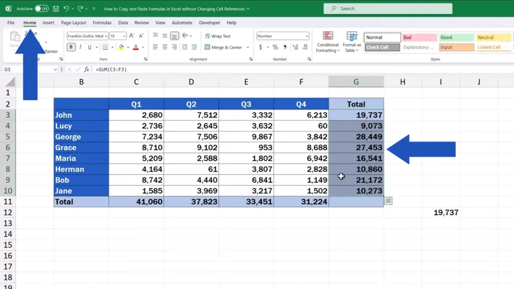
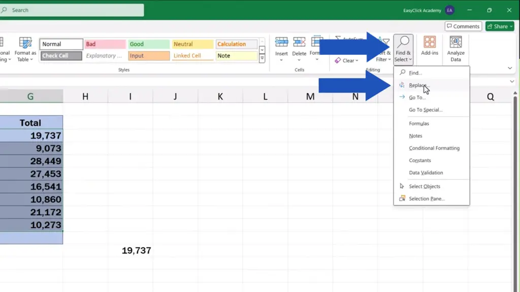
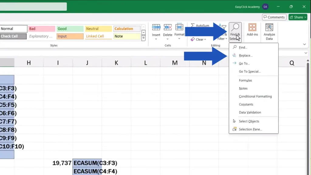
Look up ‘Find and Select’ and click on ‘Replace’.

A window pops up where we can make slight changes in the copied formula. This change will allow us to copy the formula without changing the cell references.

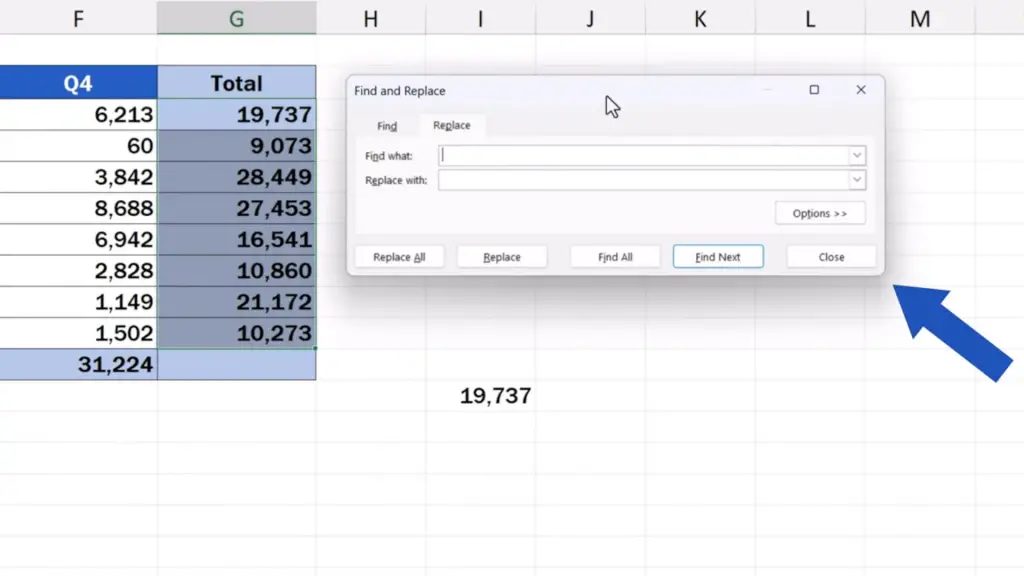
Since each formula in Excel starts with the equal sign, we need to replace this sign with another symbol or a set of symbols to turn the formula into a piece of simple text for a short while. We type the equal sign in the field ‘Find what’ and replace it with characters inserted in the field ‘Replace with’. But we need to make sure that the characters we’re about to insert are not part of any formula contained in the spreadsheet, so that all formulas would stay untouched. To do that, we can use a special set of symbols or a unique word. For this spreadsheet, we’ll replace the equal sign with the initials of EasyClick Academy. So, in the box ‘Replace with’, we’ll type ‘ECA’.

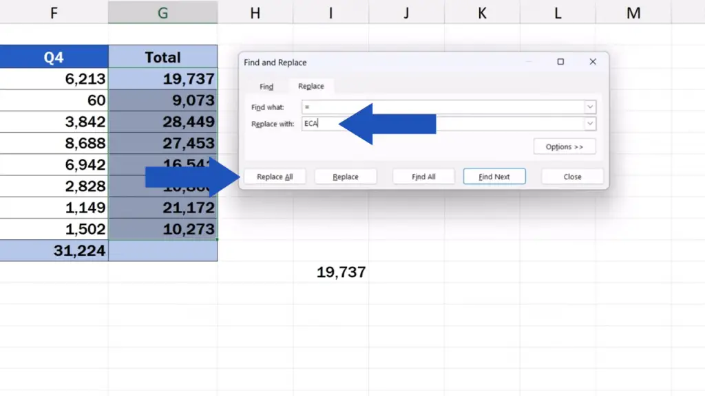
Now, when we hit ‘Replace All’, the equal sign is replaced with the letters ‘ECA’. The formulas in column G now show as plain text which can be fully copied elsewhere with the cell references unchanged, as they are considered to be part of the text.

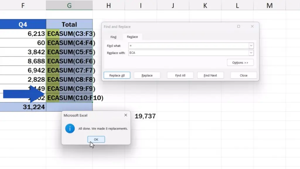
Let’s close these windows – we don’t need them at the moment, and we can move on.

Now, we can simply copy this text using Control + C and paste it in J12 using Control + V.

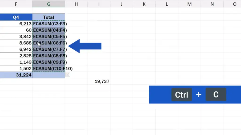
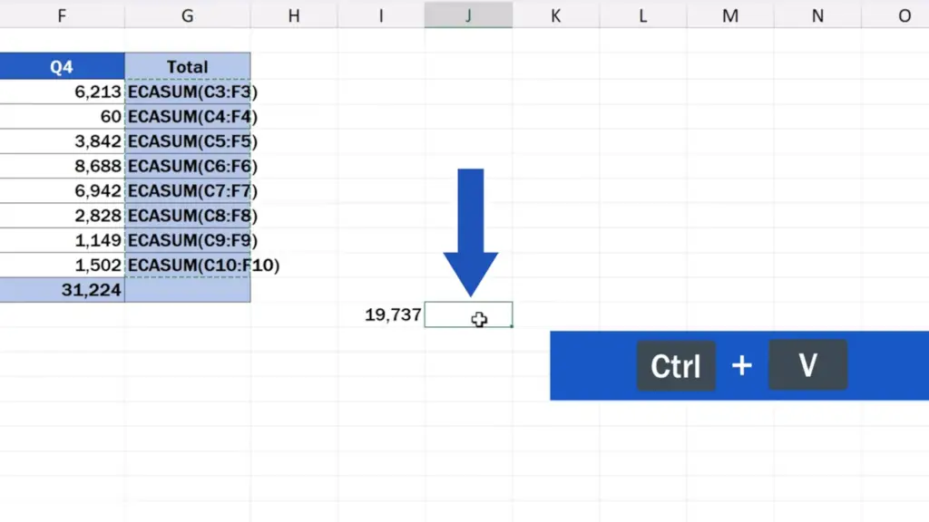
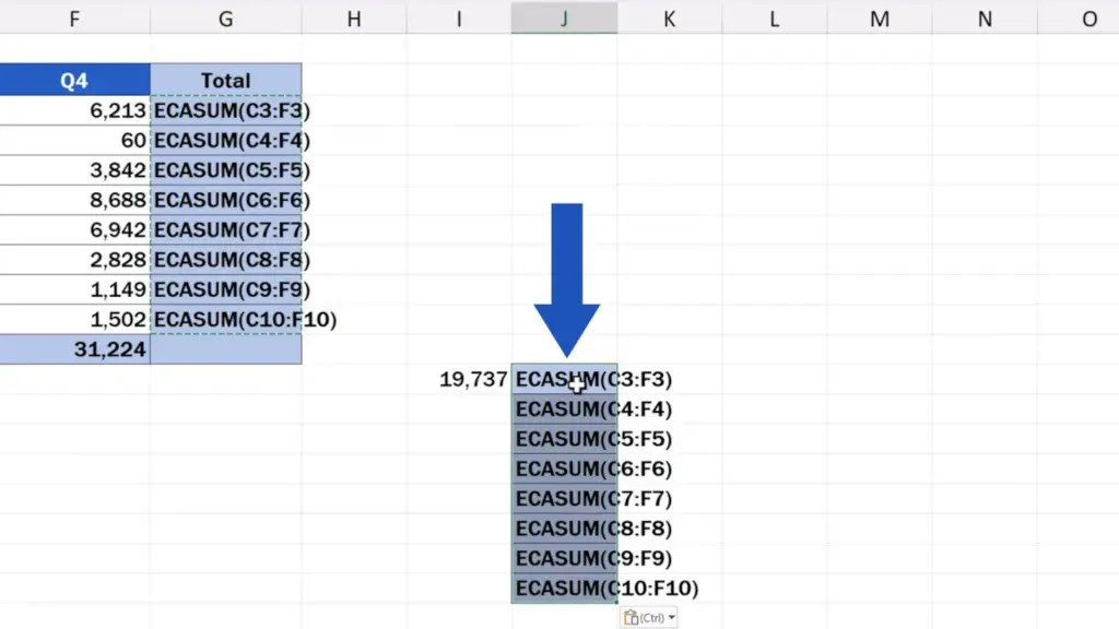
And here comes the last step: we’ve got to take the copied text and turn it into formulas again. And we’ll do so in both columns G as well as J.

Let’s not select anything now, let’s just click anywhere in the spreadsheet.

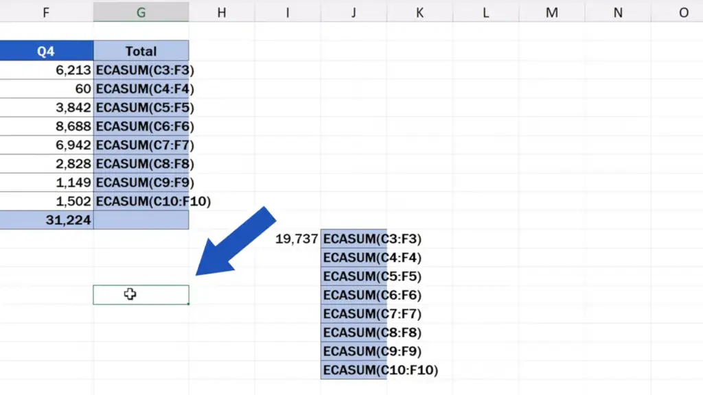
We open ‘Find and Select’ again and click on ‘Replace’.

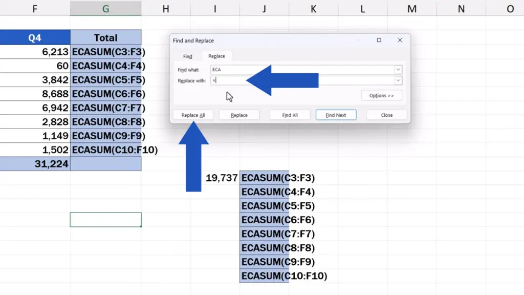
And now we do the opposite of what we did a short while ago. In the field ‘Find what’ we enter ‘ECA’ and in ‘Replace with’ we type the equal sign.

This way we’re replacing the characters ‘ECA’ with the equal sign throughout the spreadsheet to fix all the formulas. We just press ‘Replace All’ now and the formulas are working again! Let’s close the windows and check whether everything works as it should.

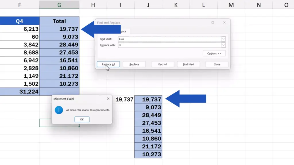
Let’s click on the cell J12 and check the formula – and we see that the formula has the same cell reference as the formula in the original cell G3. So, in both cases we get the sum of the cell range C3 to F3. The same here, in J15 – the cell references in J15 are identical to the cell references in the original cell G6.

Don’t miss out a great opportunity to learn:

• How to Copy And Paste Values Without Formula in Excel
• Shortcut Key for Paste Special in Excel

If you found this tutorial helpful, give us a like and watch other tutorials by EasyClick Academy. Learn how to use Excel in a quick and easy way!

Is this your first time on EasyClick? We’ll be more than happy to welcome you in our online community. Hit that Subscribe button and join the EasyClickers!

Thanks for watching and I’ll see you in the next tutorial!