How to Combine Cells in Excel

In this tutorial, I’ll guide you through a simple way how you can combine contents of multiple cells within one cell. This means that the times of dull copying and pasting of data bit by bit are over!

And this is how to do it!

See the video tutorial and transcription below: 

See this video on YouTube:
https://www.youtube.com/watch?v=aVb8wP5iArY

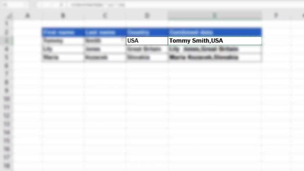
We’ll use the following example data set – first names, last names, and countries, and we’ll end up having them all written out in one cell, one next to each other, in the rows of the column E.

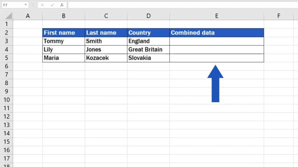
Although there are more ways to the same outcome, we’ll have a look at one, the simplest one only.

Simplest Way How to Combine Cells in Excel

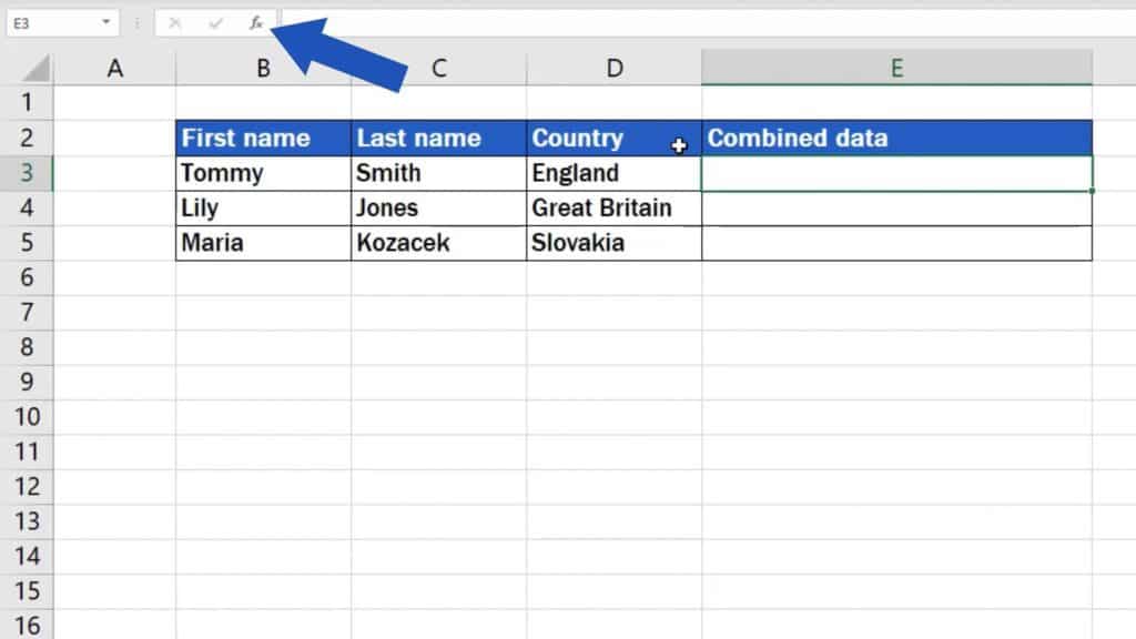
First, select a target cell that should contain the final combined contents.

Then click on the option f_x – ‘Insert Function’.

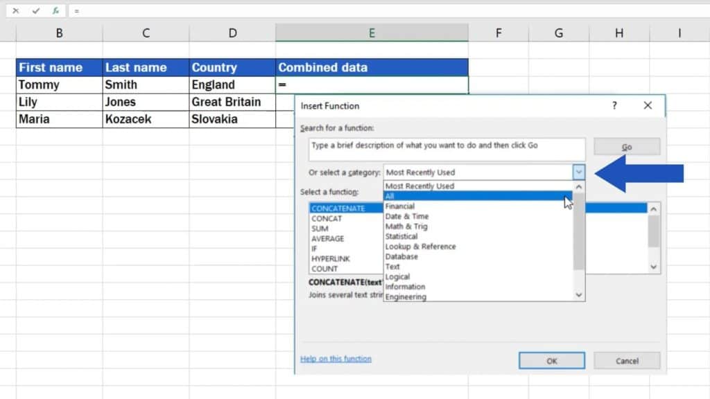
A pop-up window appears where, in the box which says ‘select a category’, we’ll choose ‘All’.

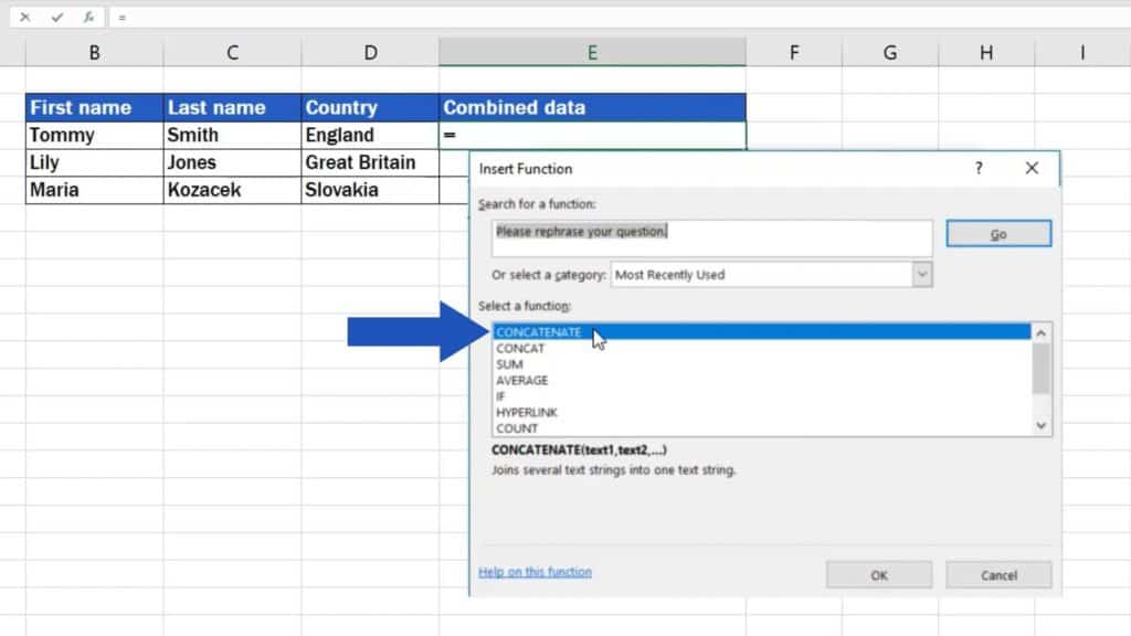
Look for the function ‘Concatenate’ and confirm with OK.

At this point, Excel will offer you only two boxes at first – Text 1 and Text 2, into which you can type the text you want to combine. More boxes are added automatically when you click into the last box. And if you still need some more – don’t worry! Excel will allow you to concatenate exactly two hundred and fifty-five text boxes like these.

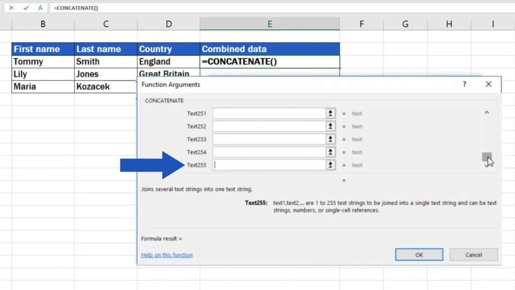
Alright then, let’s enter a first name into the ‘Text 1’ box here. We’ll click into the box with ‘Text 1’ and, right away, click on the cell which contains the data we want to use, in our case cell B3.

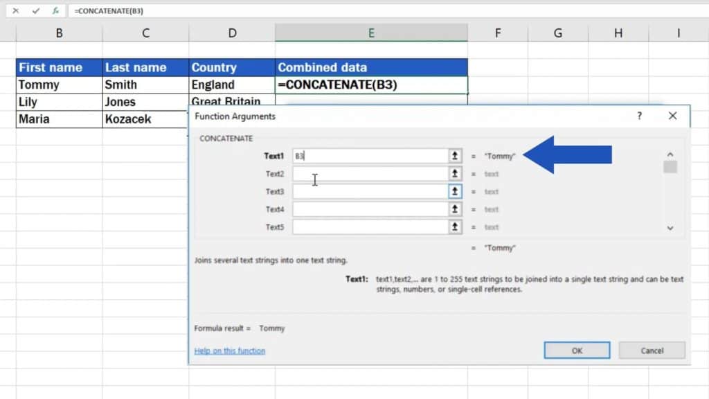
So far so good!

Now let’s say we want to add a space between the first and the last name. We’ll click into the box ‘Text 2’ and hit the spacebar to enter a single space. When we move to the box below (box number 3), Excel will turn this simple space into double quotation marks with the space located between them.

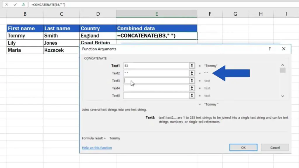
Well, let’s carry on!

The box with ‘Text 3’ should contain a last name, which means we’ll click into the box again and then click on the cell C3 which contains the ‘wanted’ bit of information. It might be very helpful to check this part over here – it displays how concatenated text will look like once done.

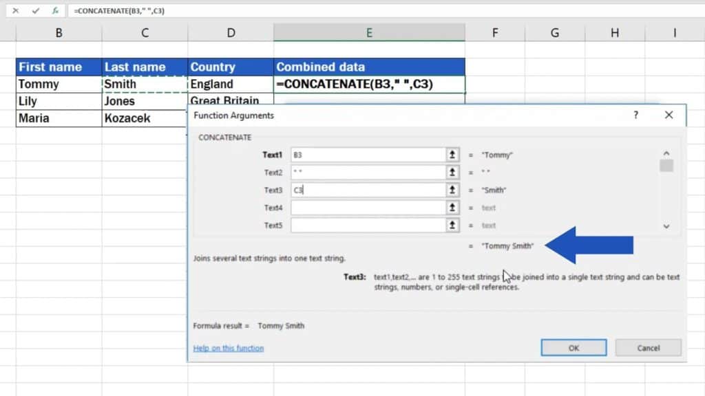
If you need to add a comma after the last name, type in a comma into ‘Text 4’ box and it immediately appears in the preview, as you can see. The same way you can add a hyphen, colon or any character you need.

And the box ‘Text 5’ will be filled in with a country. To do this we’ll follow the same steps you’re familiar with now.

Once everything we need has been combined, click on OK.

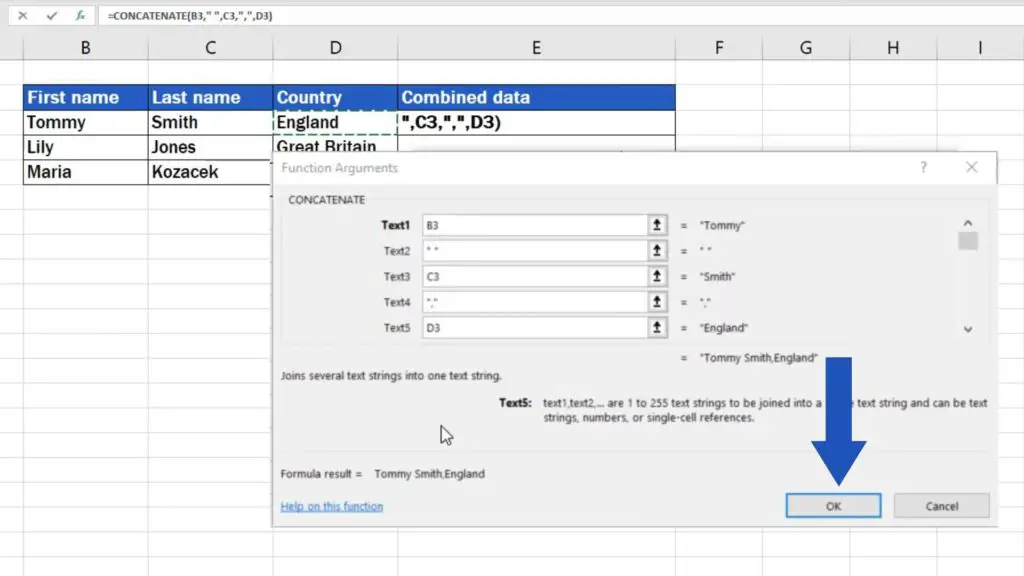
Voila! The text has been linked together without tedious copying and pasting or even retyping!

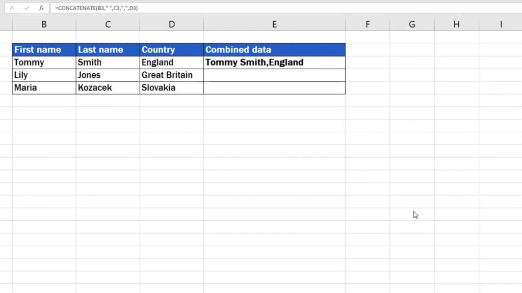
How to Combine Text in the Remaining Rows

In case you need to combine the text in the other rows, too, you don’t have to write out any functions or data again. Just hover with your mouse over the bottom right corner of the cell that contains the prepared function and drag it down through all the rows in which you want to use the ‘concatenate’ function.

Like this!

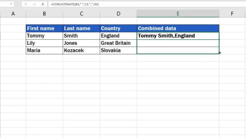
And here’s an important tip before we wrap it all up.

How to Change any Data in the Cell With Concatenated Text

Once everything has been concatenated and when you click on a cell that contains combined text, you’ll see that the cell does not contain the text itself, but references to other cells as well as spaces and commas from the final text included in quotation marks, just as is needed.

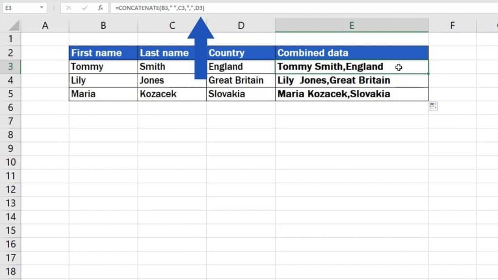
Therefore, if you want to change any data in the cell with concatenated text, you’ll need to make changes in the source cells that include this piece of information. For example, if we wanted to change England to the USA, we will do so in the column containing countries and the information will automatically change in the target cell with the final text.

Maybe you’re asking now how the concatenated text (not the formula) can be copied for further work into another cell as a simple text.

Don’t miss out the next video tutorial with us where you’ll learn:

• How to Copy And Paste Values Without Formula in Excel
• How to Separate Names in Excel

If you’ve found this tutorial helpful, like us and subscribe to receive more videos from EasyClick Academy. Look at more tutorials that help you use Excel quick and easy!

See you in the next tutorial!