How to Clear or Remove Filter in Excel

In the previous tutorial you could see how to create a filter in Excel. Today, we’ll have a look at how to clear or completely remove filter from a table.

Ready to start?

See the video tutorial and transcription below:

See this video on YouTube:  
https://www.youtube.com/watch?v=Jnn4oxSXV4g

First, we need to have a look at how to spot quickly that a filter is ‘on’ in one of the columns.

Then, we’ll go through how to clear or completely remove the filter from the table.

Let’s start from step one.

How to Recognise That Filter Is Used in Excel

If some information has been filtered out in one of the columns, you’ll recognise it by spotting a small ‘funnel’ icon in one of the drop-down buttons.

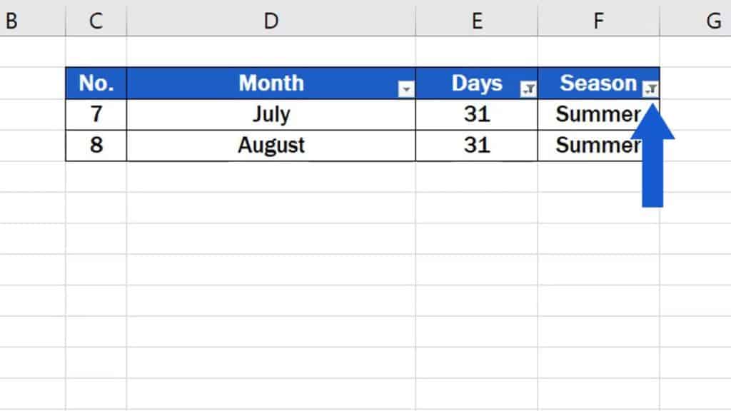
The basics of how to use a filter were shown in the previous video tutorial on how to create a filter in Excel. So here, we can see the already applied filter in the columns ‘Days’ and ‘Season’. There’s nothing similar in the column ‘Month’, which means that in that column, no data have been filtered out.

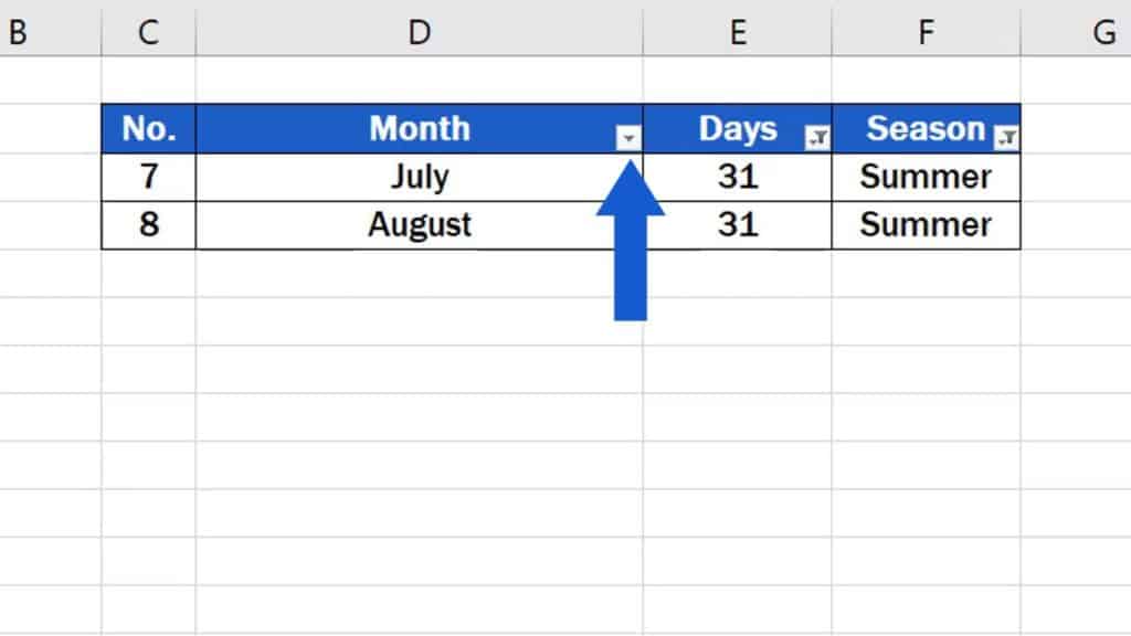
Well, we’ll carry on now and see how to clear filter in the table. And as usual, there’s more than one way to do that.

How to Clear the Filter from All Columns at Once in Excel

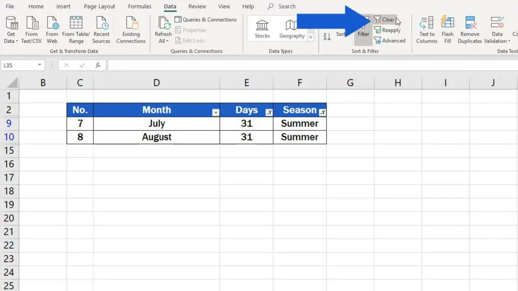
The first way is to use one click to clear the filter from all columns in the table at once. Go to ‘Data’ tab, section ‘Sort & Filter’, and find and click on ‘Clear’.

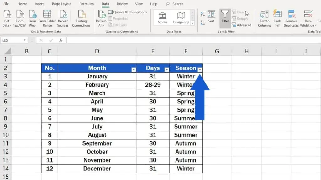
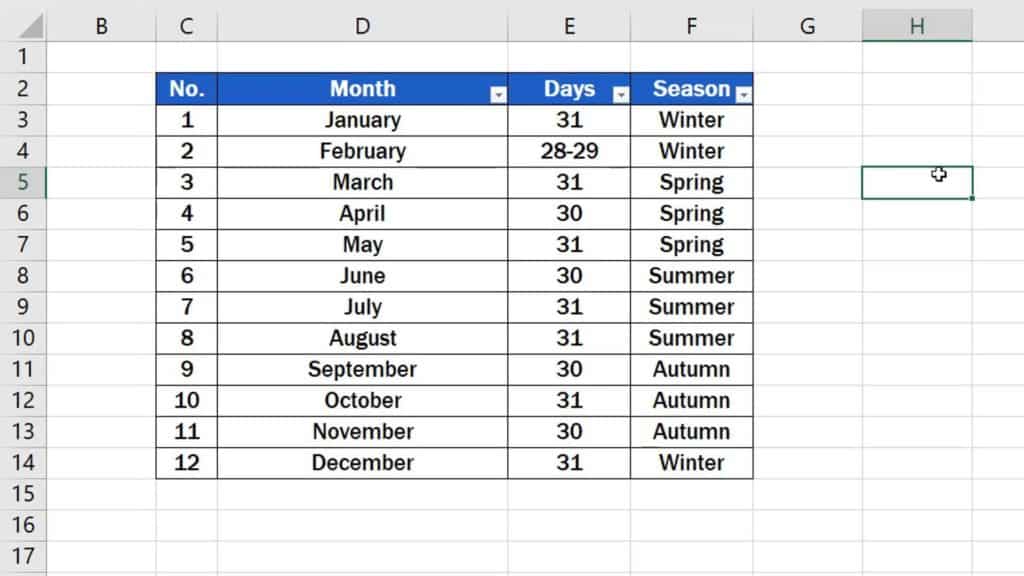
All filters from the table will be cleared in one click and all data will be visible again.

How to Turn the Filter off in Each Column Individually in Excel

The other way is convenient if you want to clear the filter column by column, not to clear it from the whole table at once. We’ll undo the last changes to turn the filter back on again, and we’ll go step by step through the whole procedure. If you want to clear the filter column by column, you’ll need to click on each drop-down button one by one and click on the option ‘Clear Filter From’,

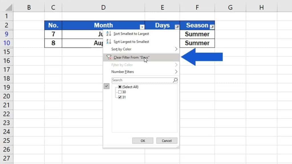
which will turn the filter off in each column individually.

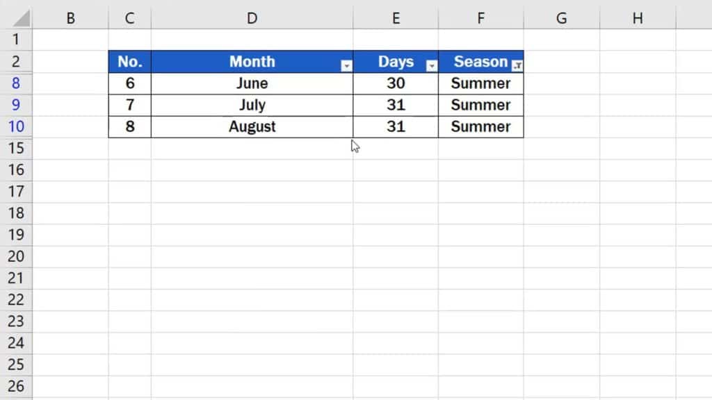
You can use this ‘column-by-column’ way to turn off all active filters in the table. Eventually, you’ll be able to see all information contained in the table again.

How to Remove the Filter from the Excel Table Entirely

And finally, if you wish to remove the filter from the table entirely along with the drop-down buttons from the column headers, it’ll be easier than you think.

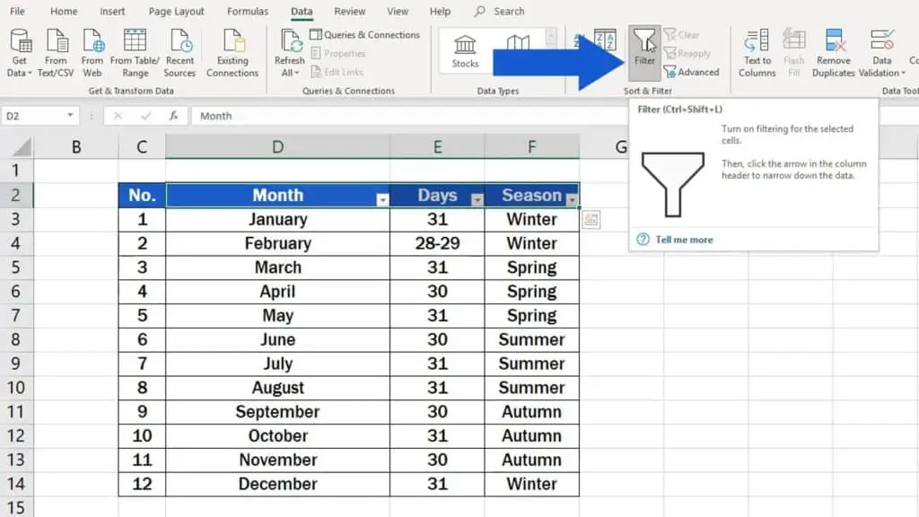
Select the cells containing the drop-down arrows,

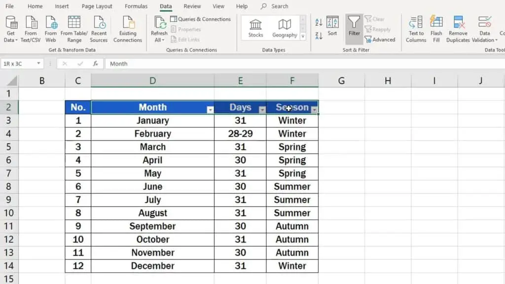
click on the ‘Data’ tab, then on ‘Filter’,

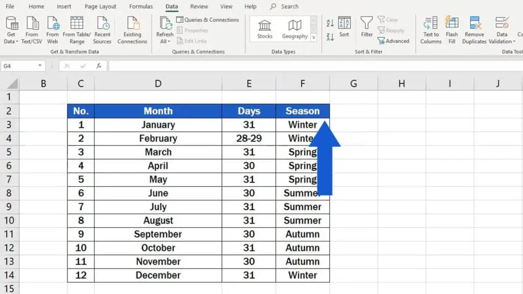
and the drop-down arrows that enable filtering are gone!

Don’t miss out a great opportunity to learn:

• How to Create Filter in Excel
• How to Create a Drop-Down List in Excel
• How to Edit Drop-Down List in Excel

If you found this tutorial helpful, give us a like and watch other video tutorials by EasyClick Academy. Learn how to use Excel in a quick and easy way!

Is this your first time on EasyClick? We’ll be more than happy to welcome you in our online community. Hit that Subscribe button on our YouTube channel and join the EasyClickers!

See you in the next tutorial!