How to Change Row Height in Excel

In this tutorial, we’ll cover how to change the height of a row in Excel in a super easy way.

Keep watching! We’re about to start.

See the video tutorial and transcription below: 

See this video on YouTube:
https://www.youtube.com/watch?v=r3Sx-awB_-A  

As you might’ve already noticed, Excel usually offers more than one solution to any task. The same applies when it comes to changing the height of a row in a spreadsheet. In a couple of seconds, we’ll guide you through the two quickest and easiest ways to do this.

First Quick Way How to Change Row Height in Excel

Sometimes, you need to adjust the row height but don’t know the exact dimensions or value, in points, to specify the height. In that case, follow these steps:

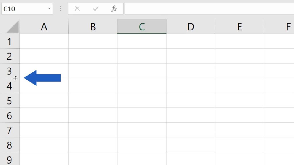
Position the cursor at the bottom border of the row whose height you need to change. Once the cursor turns into this double-headed arrow,

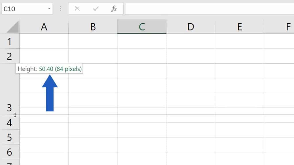
left-click and drag the arrow to adjust the height of the row as needed. While dragging, this box will show you the current row height in figures, so you’ll be able to follow number values, too.

And now the other way.

Second Quick Way How to Change Row Height in Excel

Imagine that you know the exact number of points to enter to adjust the row height. Here’s what you do.

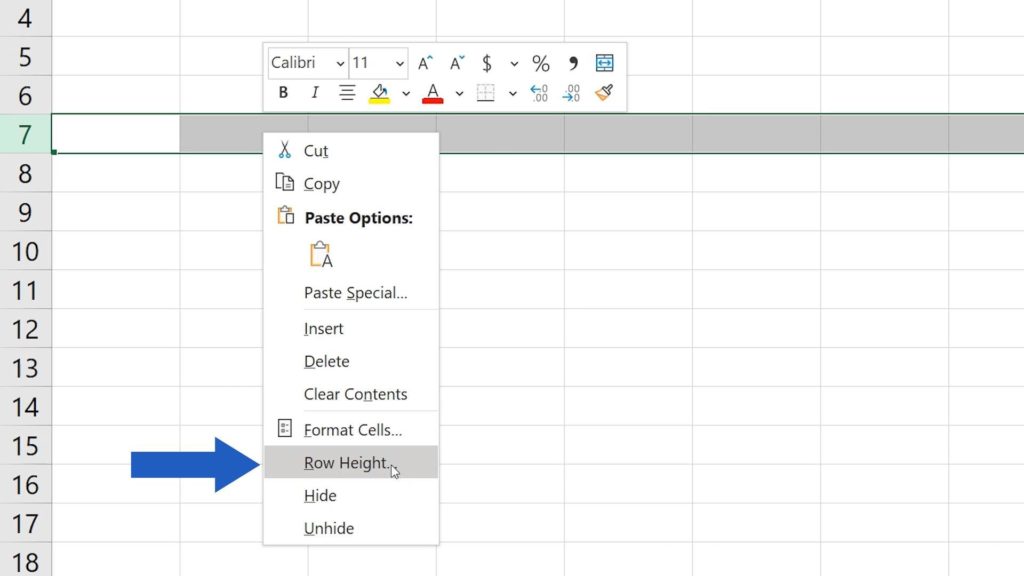
Click on the row to select the area  – let’s say we need to change the height of the row 7 here. Right-click on the row and choose the option ‘Row Height’.

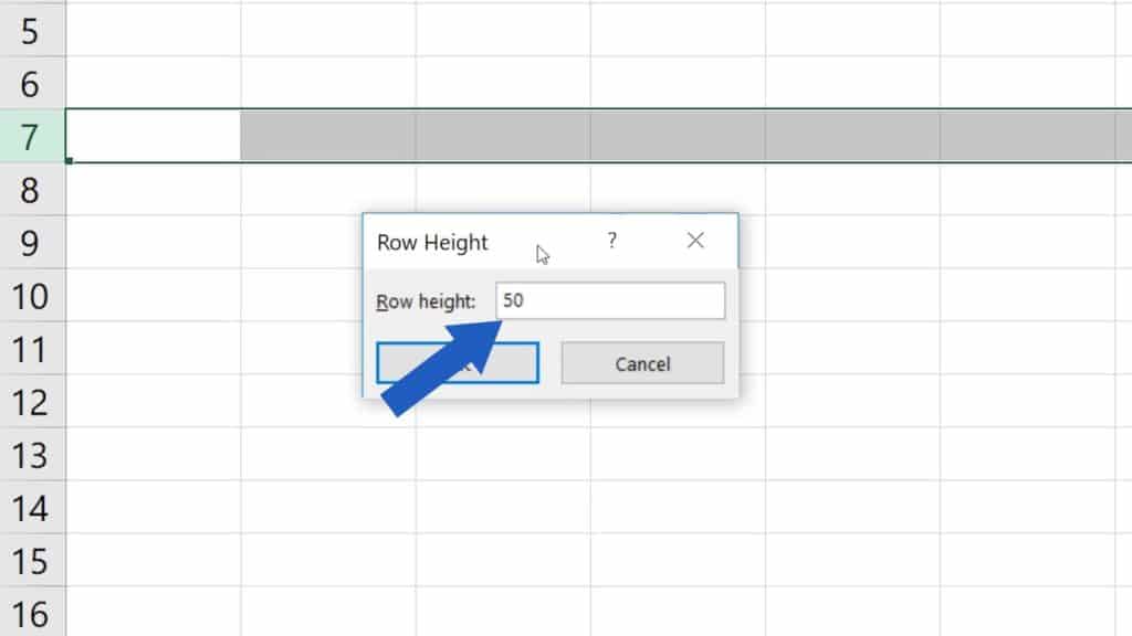
Now simply enter the value for the height, for example 50. Click on OK and it’s done!

How to Change Height of Multiple Rows in Excel

You can easily use the same way to change the height of multiple rows at once.

If you’d like to see more on how to work with rows in Excel, check out the links the description below!

• How to Hide Rows in Excel
• How to Unhide Rows in Excel
• How to Delete Row in Excel
• How to Insert Row in Excel
• How to Freeze a Row in Excel

Is this your first time on EasyClick? We’ll be more than happy to welcome you in our online community. Hit that Subscribe button and join the EasyClickers!

Thanks for watching and I’ll see you in the next tutorial!