How to Change Lowercase to Uppercase in Excel

In today’s tutorial we’re going to go through how to change lowercase to uppercase in Excel and we’ll be talking about cells containing the mix of upper- and lower-case letters, too.

Let’s start!

Would you rather watch this tutorial? Click the play button below!

How to Change Lowercase to Uppercase in Excel

If you’d like to change lowercase letters in a cell to uppercase, click on the cell to select it first. Then type in the equal sign and start typing out the function ‘UPPER’.

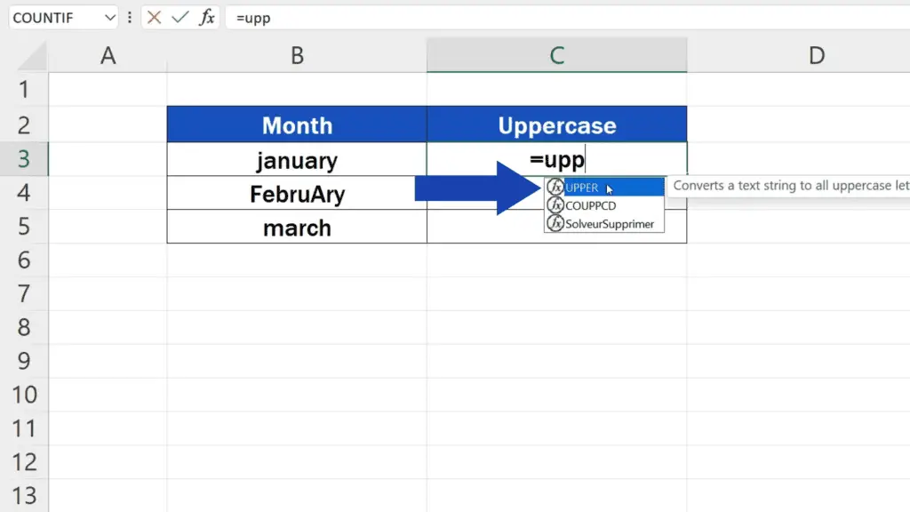
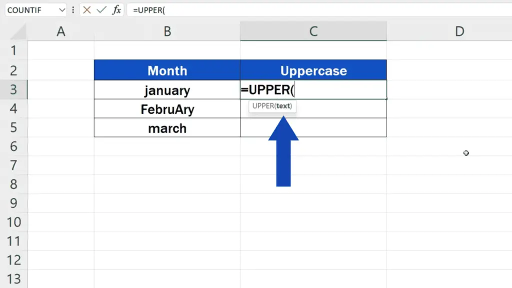
Click on the suggestion and carry on by defining the cell that contains the text you’d like to convert into uppercase.

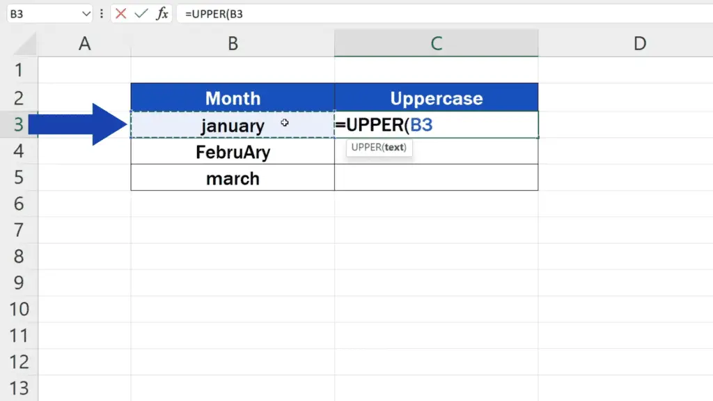
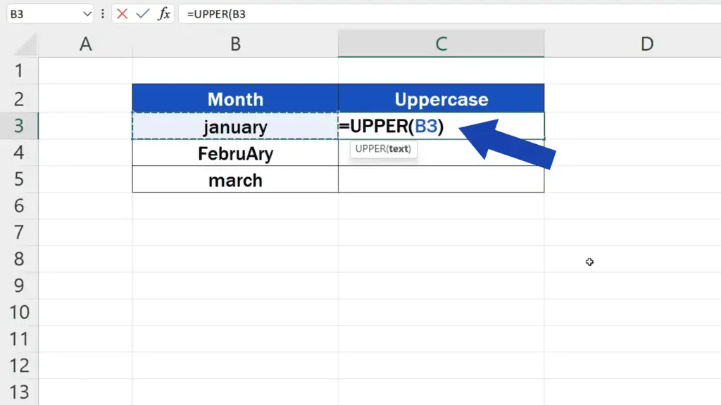
Here it is the text in the cell B3, so we’ll click on B3, close the brackets, press Enter and here we go – all uppercase now!

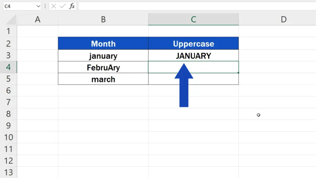
How to Copy the Function to the Rest of the Rows

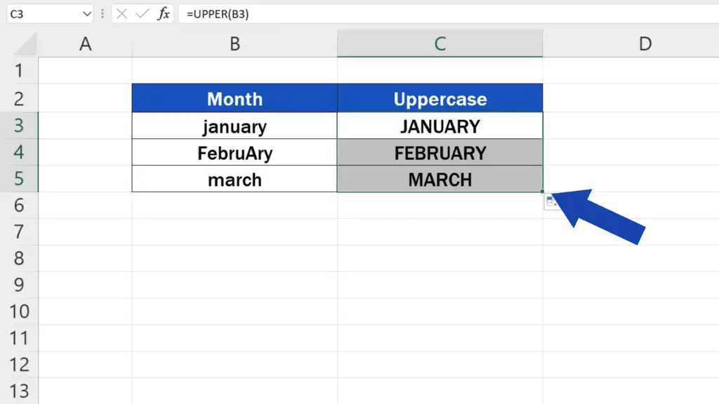
If needed, you can copy the function through drag and drop to the rest of the rows and change the lowercase letters into uppercase for all the data.

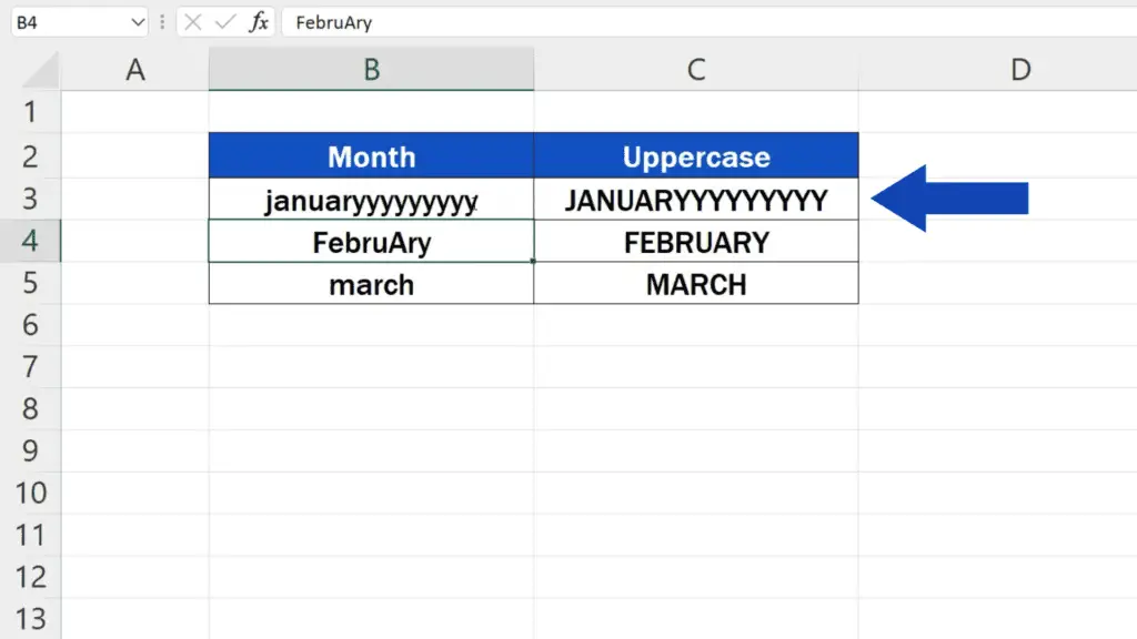
Now, if you change anything in the source cell, the change will be reflected in the converted text.

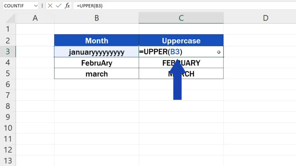
This happens because we used a function to convert the text into uppercase, which we can see if we click into the cell C3.

But what if we need to store only the values, the converted texts themselves, and we don’t want to keep the function in the data table? Well, that’s easy to do.

How to Store Only the Values in the Cell

Let’s select the converted data and use the control key [Ctrl] and C to copy the contents of the cells.

Now, we use ‘Paste’ here at the top to simply paste them in the same place, but we need to go for the option ‘Values’.

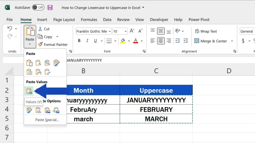
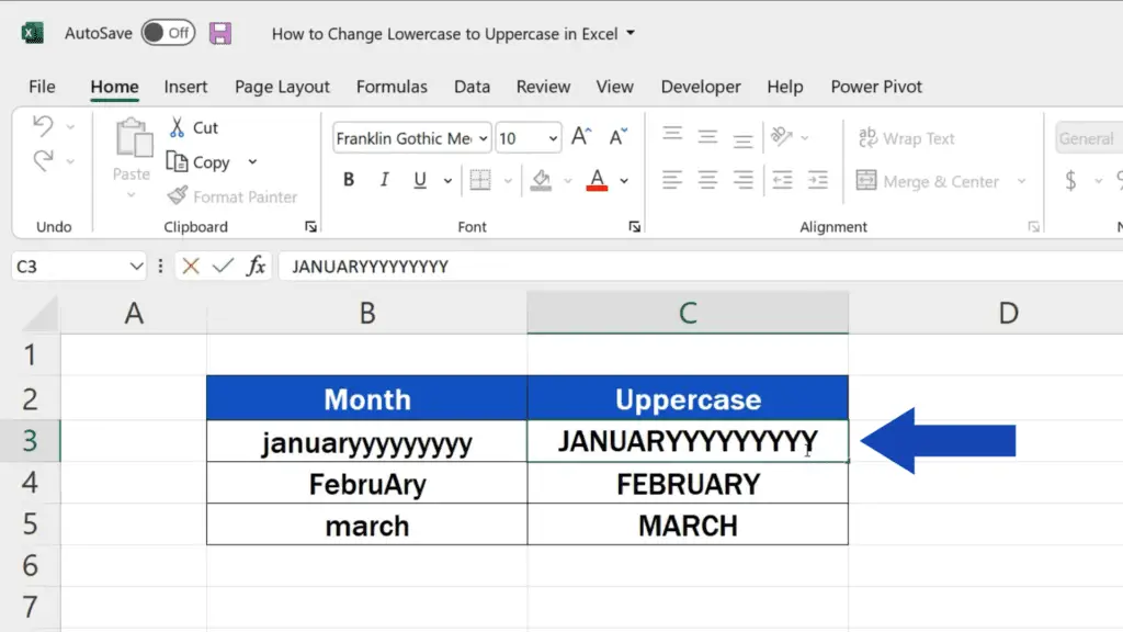
Through this we make sure that all the cells contain the converted text only.

Don’t miss out a great opportunity to learn:

• How to Change Capital Letters to Lowercase in Excel
• How to Change Text Direction in Excel
• How to Replace Words in Excel (and avoid unnecessary mistakes

If you found this tutorial helpful, give us a like and watch other tutorials by EasyClick Academy. Learn how to use Excel in a quick and easy way!

Is this your first time on EasyClick? We’ll be more than happy to welcome you in our online community. Hit that Subscribe button and join the EasyClickers!

Thanks for watching and I’ll see you in the next tutorial!