How to Calculate Discount Percentages in Excel (Quick and Easy)

Today we’ll be talking about how to calculate discount percentages in Excel in a quick and easy way.

Let’s get into it right now!

Would you rather watch this tutorial? Click the play button below!

How to Format the Cell as Percentage

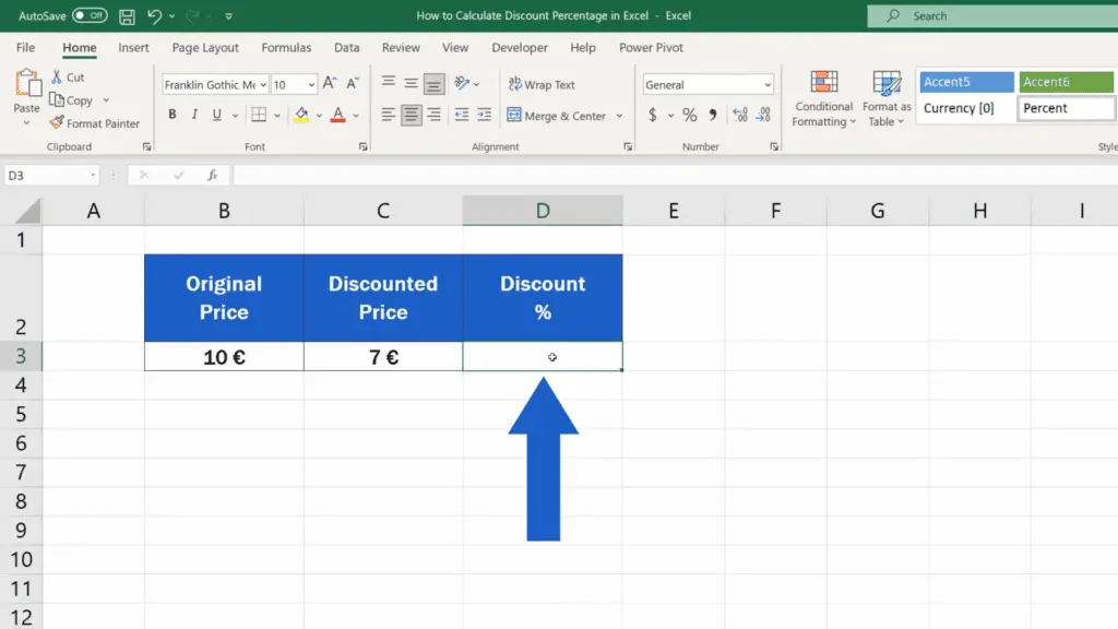
To calculate a discount percentage in Excel, first select the cell where you’re planning to show the result.

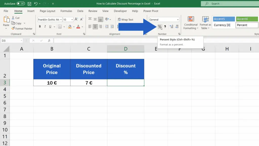
Then go to the Home tab and format the cell as Percentage using this ‘Percent Style’ button. This way you’ll make sure Excel will display the results as a percentage, including the per cent sign.

How to Calculate Discount Percentages

Once the cell has been formatted correctly, we type in the equal sign and divide the discounted price in C3 with the original price – the price before the discount was applied – in B3.

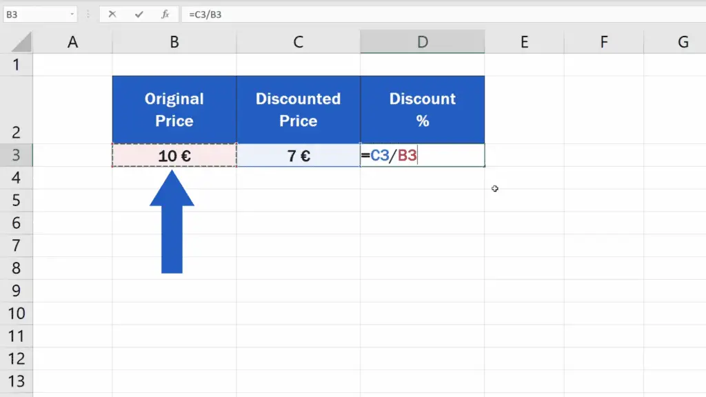
When we press Enter, we get the first important result, which tells us that the discounted price (7 euros) is 70% from the original price of 10 euros.

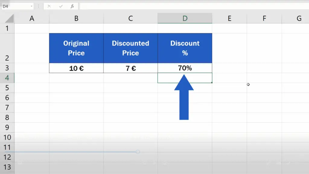
However, we’re trying to calculate the discount, so we need to subtract this calculated figure (70%) from 100%.

In terms of the formula, we need to subtract the first result from the number 1.

So, this is the final formula, which will help you calculate the discount percentage in a quick and easy way.

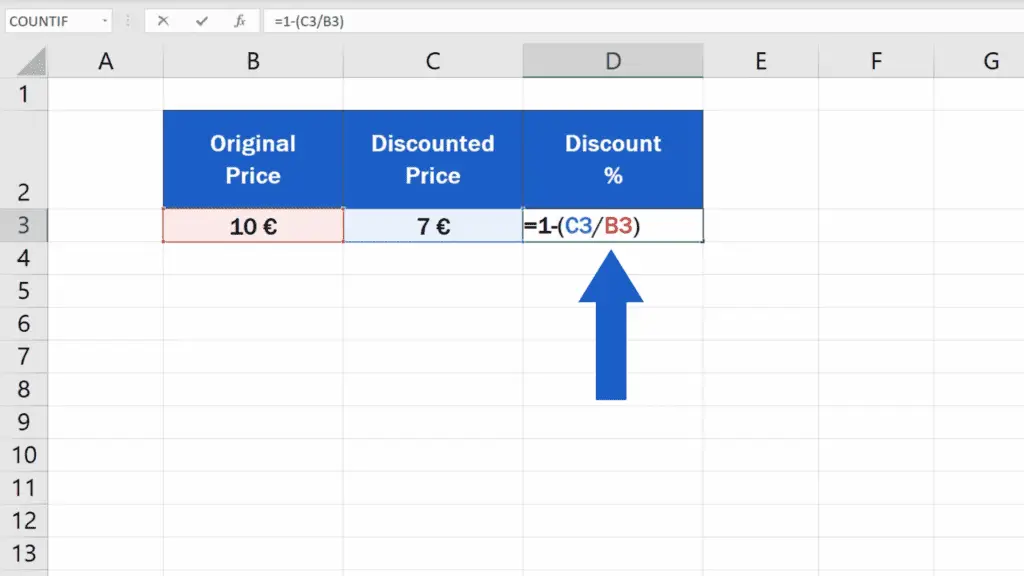
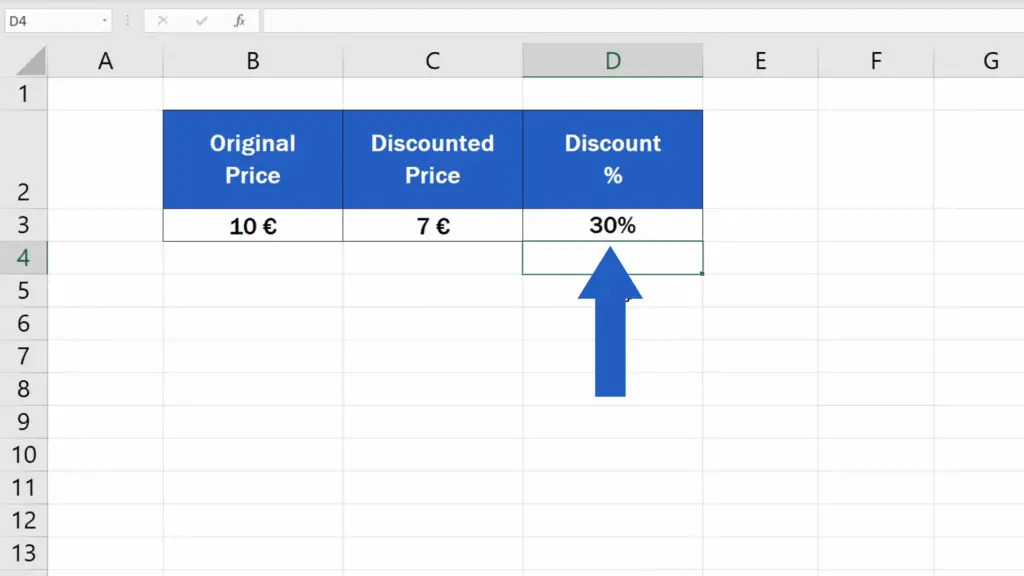
If the original price was 10 euros and the discounted price is 7 euros, you saved 30%.

And if the discounted price changes to 9 euros, Excel automatically recalculates the discount percentage and shows 10% in the target cell.

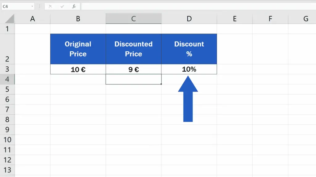
The formula works with all numbers and you’ll get the result immediately – couldn’t be quicker and easier!

Don’t miss out a great opportunity to learn:

• How to Calculate Percentage Increase in Excel (The Right Way)
• How to Square a Number in Excel (Two Most Common Ways)
• How to Get Stock Prices in Excel (Free and Automated Solution)

If you found this tutorial helpful, give us a like and watch other tutorials by EasyClick Academy. Learn how to use Excel in a quick and easy way!

Is this your first time on EasyClick? We’ll be more than happy to welcome you in our online community. Hit that Subscribe button and join the EasyClickers!

Thanks for watching and I’ll see you in the next tutorial!