How to Calculate an Average in Excel

This tutorial will show you how to calculate an average in Excel, thanks to which you’ll be able to work out an average value of a group of numbers of any size.

This function is very handy, so let’s find out together how to use it!

See the video tutorial and transcription below:

See this video on YouTube:
https://www.youtube.com/watch?v=lDjdTQt93Pc 

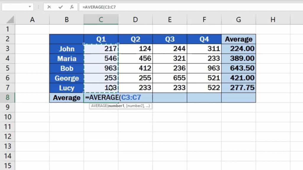
We’ll use the data in this table to see how we can calculate a mean value in Excel, using the practical function called ‘Average’.

Imagine you need to find out how many sales per quarter, but also per employee, were made on average throughout the last year.

As you already know, we must start with clicking on the cell where we want the result to appear.

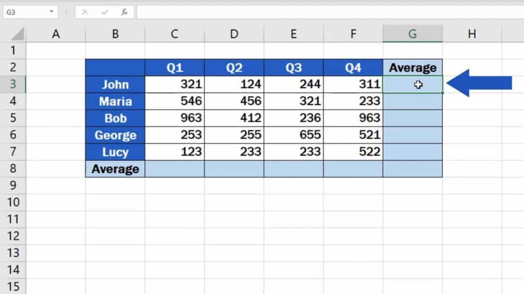
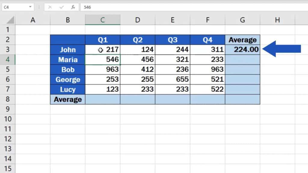
In this case we’ll use the cell G3. Here we’ll get the average value of the number of sales John made for all four quarters.

Type in the ‘equal’ sign and start typing the word ‘Average’. Excel will immediately offer various similar functions that start in the same letters. If you want to calculate the standard average value, double-click on ‘Average’.

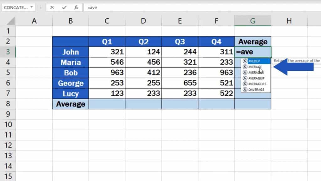
Now, you need to specify the group of numbers from which you want to calculate the average.

So, we’ll click on cell C3, then hold and drag until we reach the location F3. This way, Excel receives the information that these are the numbers that need to be included for the calculation of the average.

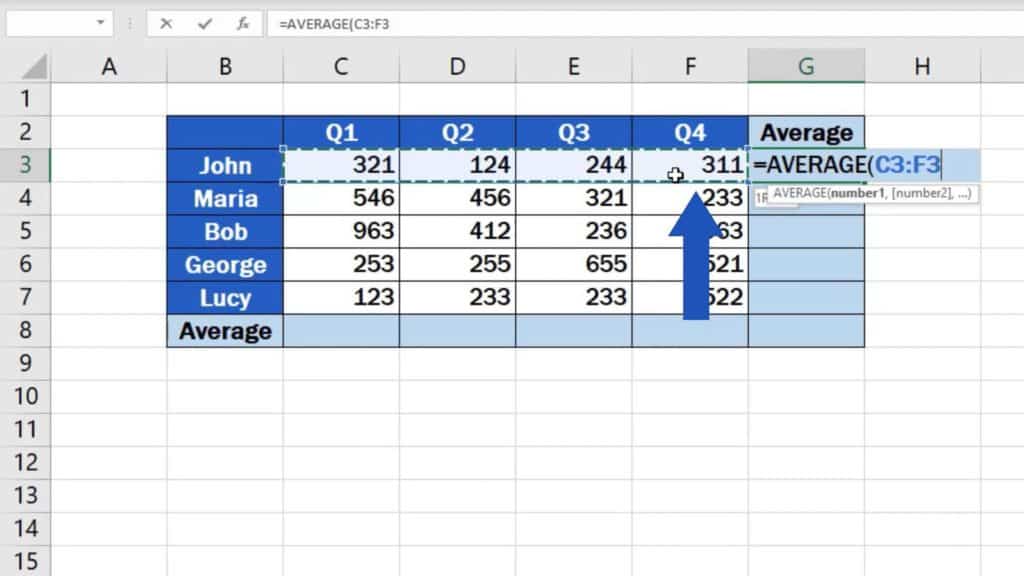
Of course, instead of clicking and dragging, you can simply type the range of selected cells into the brackets within the ‘Average’ function directly. Include the reference to the starting point of the range as cell location, then insert a colon, and right after that, type the reference to the last cell we need to include in the calculation.

Once done, press ‘Enter’ and have a look.

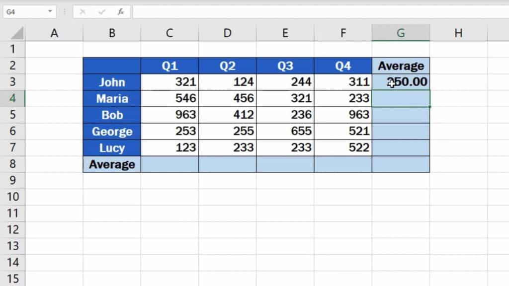
The function helped us calculate the average number of sales John made per quarter.

Actually, we would come up with the same result if we summed up the figures of John’s sales for all quarters and then divide the total with the quarter count, which is four.

However, the function ‘Average’ makes the calculation a lot quicker and easier!

But you need to be aware of one thing – if you change data in the selected range of cells, the ‘Average’ function recalculates the result automatically. For example, if you overwrite the Q1 value 321 with the number 217, the average will change, which will reflect in the target cell. So, the result will always be up to date.

And we’re not quite at the end yet!

How to Calculate the Average Number of Sales for Other People

If we need to calculate the average number of sales per quarter for other people in the table, it’s an absolute doddle.

Click on the cell containing the formula, place the pointer to the right bottom corner to see a little plus sign.

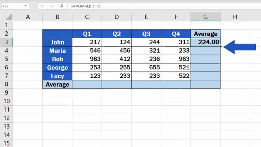
Click and hold the left mouse button and drag through all the cells where you need the formula to calculate the averages.

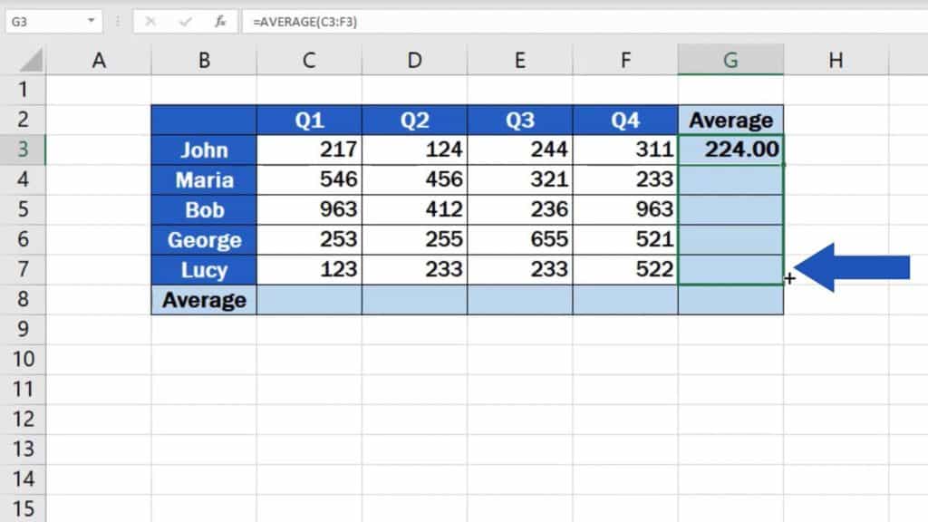
Easy, right? The average values per quarter have now been calculated for other employees, too.

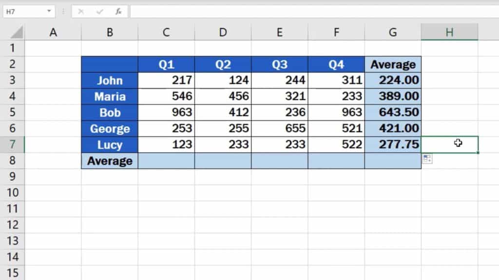
You can use the same way to calculate the average per employee for each quarter in individual columns. The formula works with any group of cells you need.

Don’t miss out a great opportunity to learn:

• How to Calculate Hours Worked in Excel
• How to Calculate Hours Worked in Excel (Midnight Span)
• How to Sum Time in Excel

Are you interested in:

• How to Add Numbers in Excel (Basic way)
• How to Subtract Numbers in Excel (Basic way)
• How to Divide Numbers in Excel (Basic way)
• How to Multiply Numbers in Excel(Basic way)

If you found this tutorial helpful, give us a ‘like’ and watch other video tutorials by EasyClick Academy. Learn how to use Excel in a quick and easy way!

Is this your first time on EasyClick? We’ll be more than happy to welcome you in our online community. Hit that Subscribe button on our YouTube channel and join the EasyClickers!

See you in the next tutorial!