How to Calculate a Rank in Excel (Descending / Ascending)

In this tutorial, we’re going to have a look at how to calculate a rank in Excel. Based on the calculation, you’ll be able to compare data of any size and determine their position within the data group.

Ready to dive in?

Would you rather watch this tutorial? Click the play button below!

How to Calculate a Rank in Excel

To rank data, first we need to click into the cell where we want to display the result.

We start typing the equal sign and the first letters of the word ‘RANK’, and Excel will come up with the right function suggestion immediately.

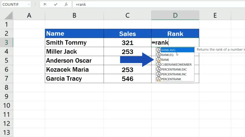
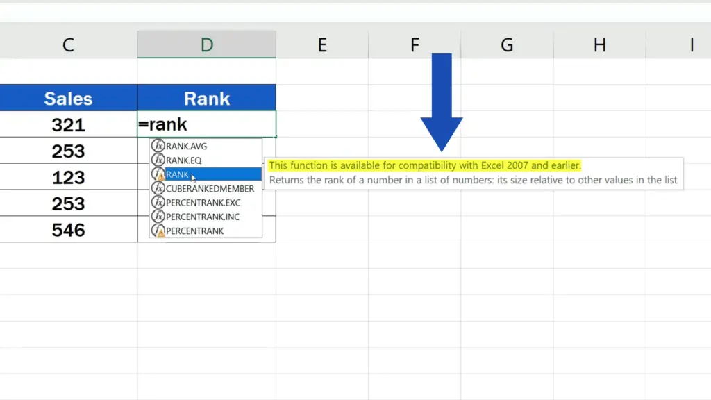
Here we need to note that the Rank function is available for compatibility with Excel 2007 and earlier.

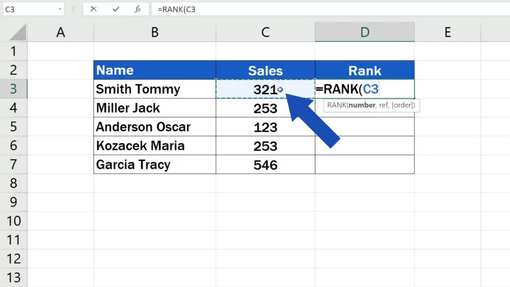
Let’s click on the suggested function and fill in the missing bits. First, we need to enter the number we want to calculate the rank for. This value is stored in the cell C3, which contains the information on Tommy’s sales.

We can add a comma and now we need to include all the numbers of the data set which we want to compare and evaluate, and against which we want to determine Tommy’s position within the ranking. So, here we’ll select the sales by the rest of the salesmen.

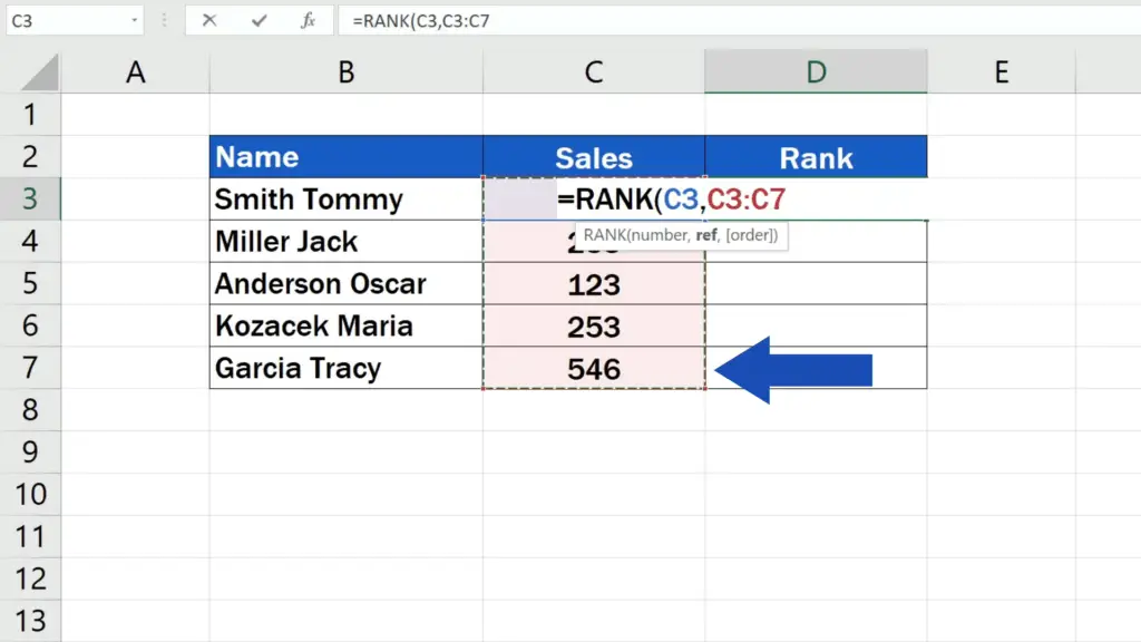
However, we need to be careful not to forget to lock the reference to this set of data. Click on C3 and press and hold the Function key along with F4. Some of you don’t have to use the Function key – this depends on the keyboard type you’re using.

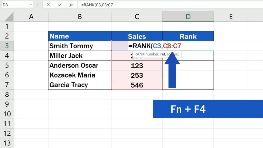
The dollar sign appeared next to the cell reference, which means that the value for calculating the rank will stay the same once the function is copied in the rows below.

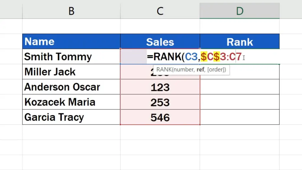
We use the same keys to fix the coordinates C7 to make sure that the reference to the whole area will remain unchanged.

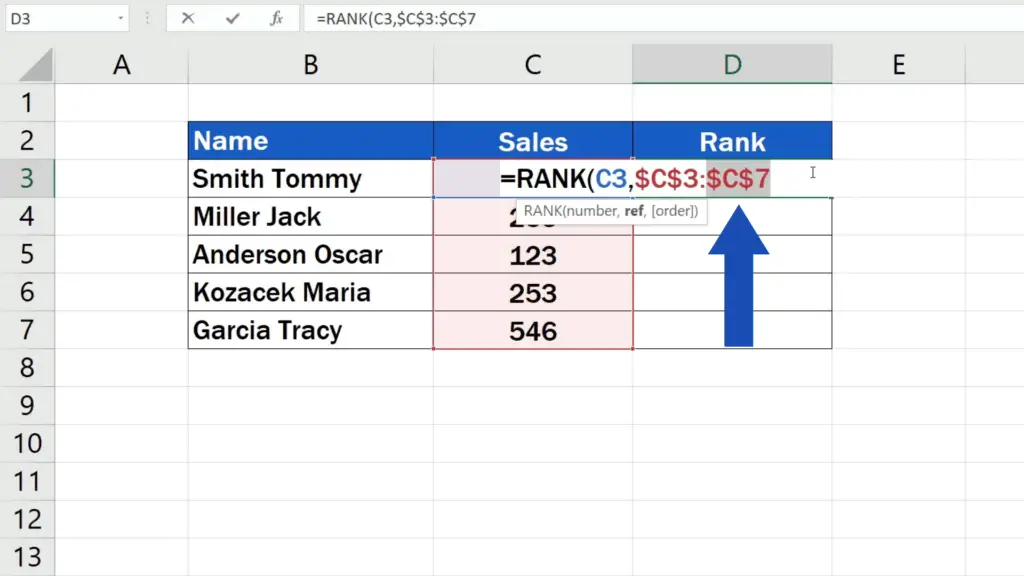
If we copy the Rank function to the rest of the rows below, the reference to the relevant cells won’t change, which is important as we want to find out the rank for each of the salesmen, so we need to keep the set of data the same in each calculation. If you’re interested to know more on how to use the absolute cell reference in Excel, check out a separate tutorial the link to which is in the list below.

How to Specify the Rank to Be Descending or Ascending

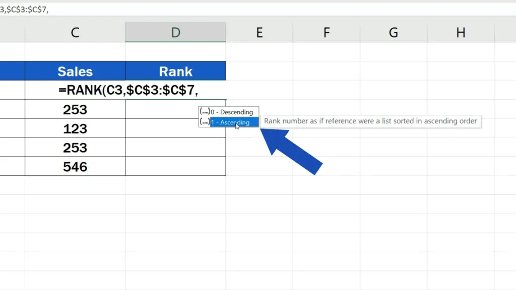
But let’s move on now and add another comma. Now it’s time to specify whether we want the rank to be descending or ascending.

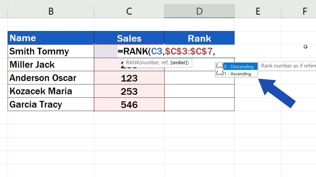
If we go for descending, the highest number on the list will become number one and the lowest sales count will be the last in the rank. This option is set as default in Excel, so if we close the bracket at this point, without adding any extra information, Excel will go on and calculate a descending rank.

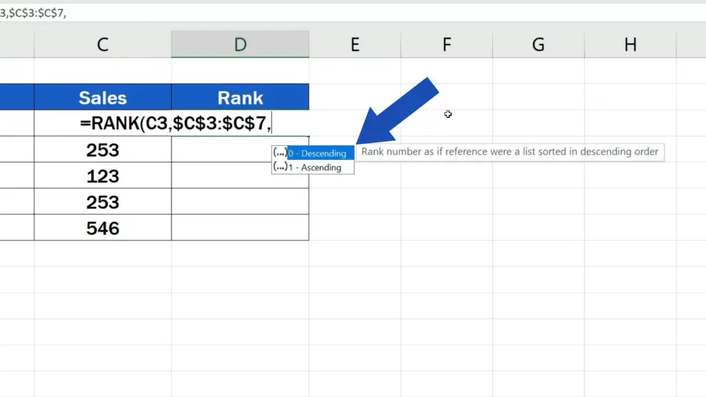
To calculate the ascending rank, we need to choose the option ‘ascending’. In that case, the lowest number will become number one and the highest number will be marked as the last in the ranking.

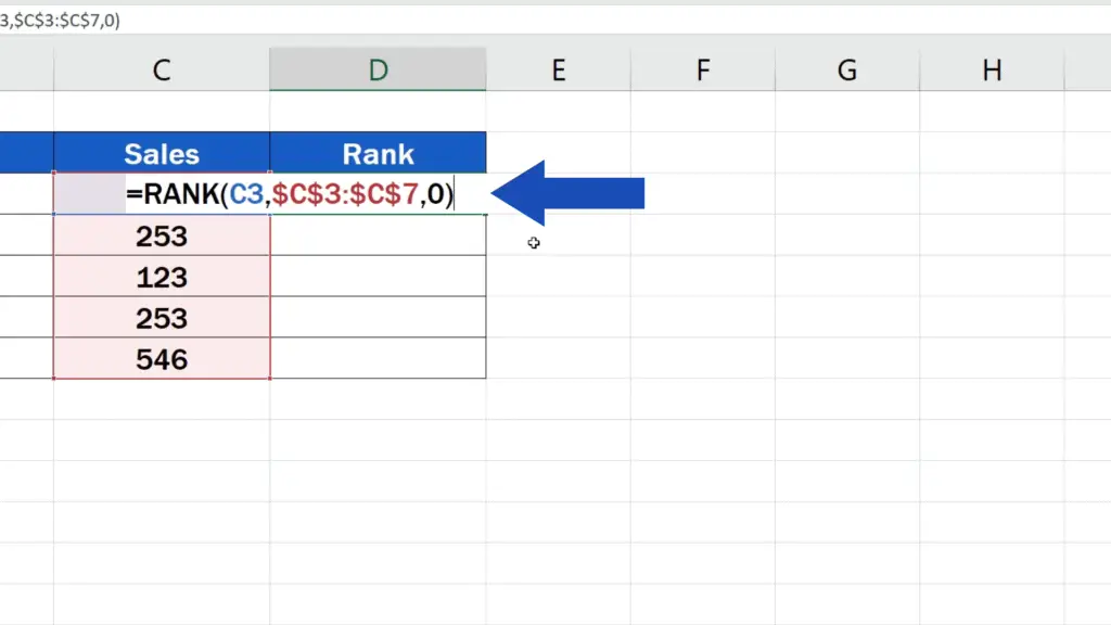
Let’s go for ‘descending’ now – click on it, close the brackets, hit Enter and here we are! You can see the position of Tommy’s sales compared to the sales by the rest of the salesmen.

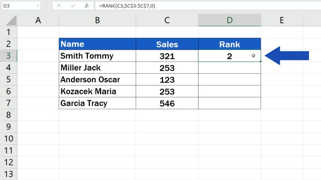
Copy the function simply by dragging the bottom right-hand corner of the cell containing the complete formula and the ranking for other salesmen appears right away.

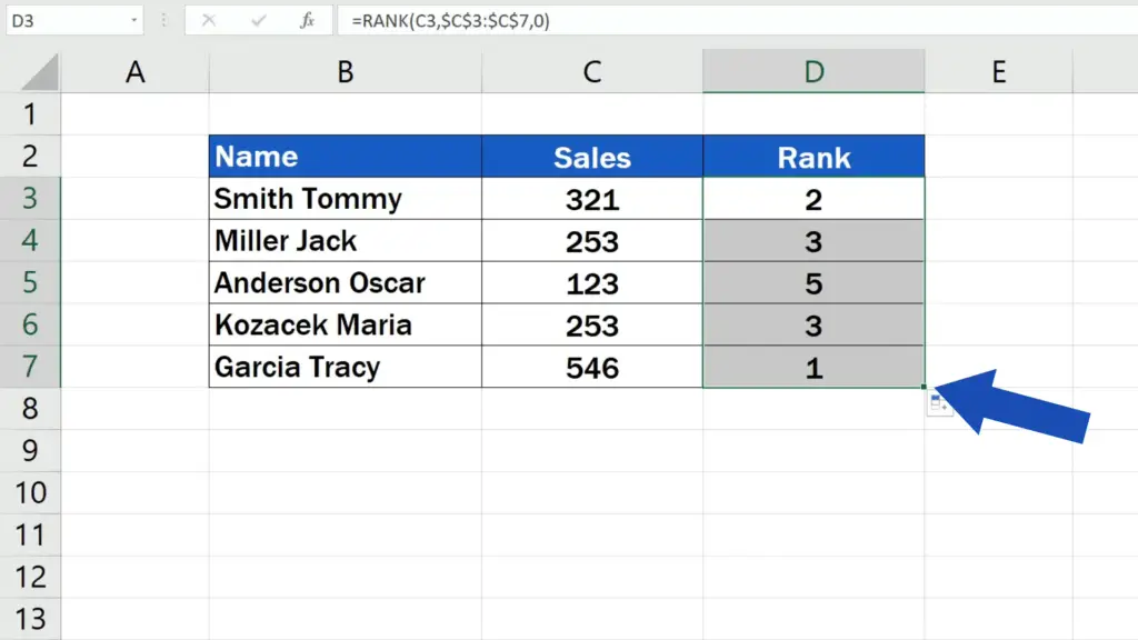
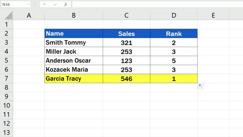
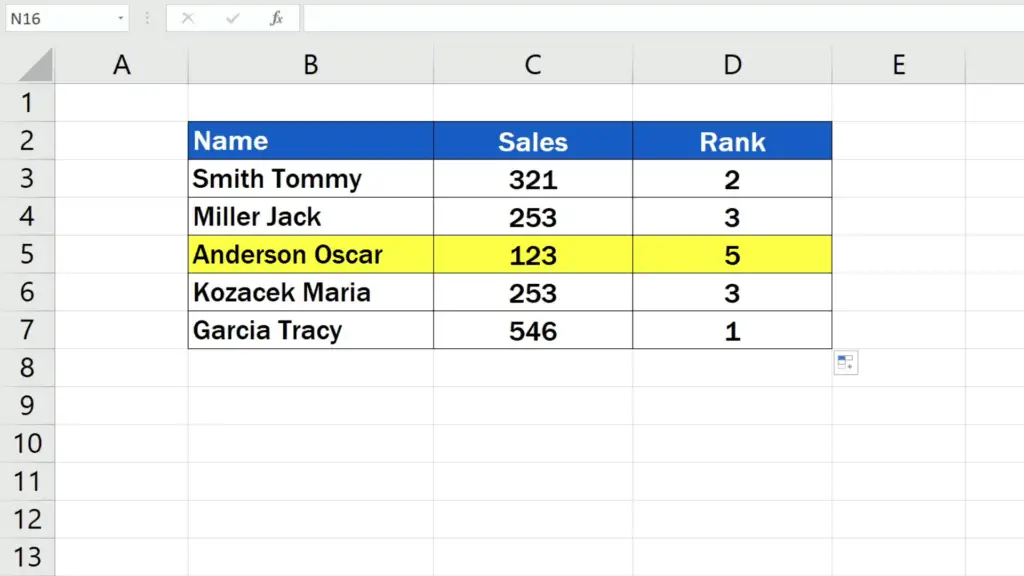
As you can see, the first one in the ranking is the salesman who got the highest number of sales and the last one is the one with the lowest sales count, just as we wanted.

How to Calculate a Rank in Excel If There Are Two Values which Are the Same

There’s one important thing to be aware of – if there are two values which are the same within the selected data area, Excel will do the evaluation in a specific way.

Here you can see that the third position belongs to two salesmen with the same sales counts. They’ve been both put in the same rank, which is three, but since there are two people with the same numbers, Excel skipped position four and the ranking continues with position five.

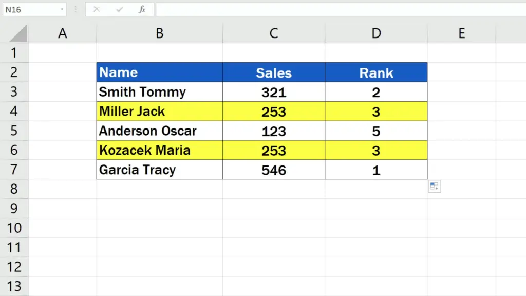
If there were three identical values on the same position, the following two places would get skipped, so make sure to keep this rule in mind when calculating a rank in Excel.

Don’t miss out a great opportunity to learn:

• How to Use Absolute Cell Reference in Excel
• How to Use SUMIF Function in Excel (Step by Step)
• How to Calculate an Average in Excel

If you found this tutorial helpful, give us a like and watch other tutorials by EasyClick Academy. Learn how to use Excel in a quick and easy way!

Is this your first time on EasyClick? We’ll be more than happy to welcome you in our online community. Hit that Subscribe button and join the EasyClickers!

Thanks for watching and I’ll see you in the next tutorial!