How to AutoFit Columns in Excel (The Simplest Way)

In this video tutorial, we’re going to have a look at the simplest way how to autofit columns in Excel. You’ll be able to easily amend column width, so that the width of each column will be the narrowest possible but showing all data at the same time.

Ready to start?

How to Select Multiple Columns for Autofit in Excel

There are a number of ways to autofit columns in Excel. Let’s take a look at the simplest one now!

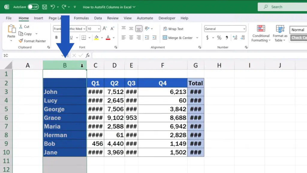
First, we select all the columns we want to autofit. Here, we click on column B.

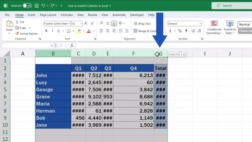
And hold the left mouse button while dragging the cursor through to column G. This way we’ve selected all the columns in this data table.

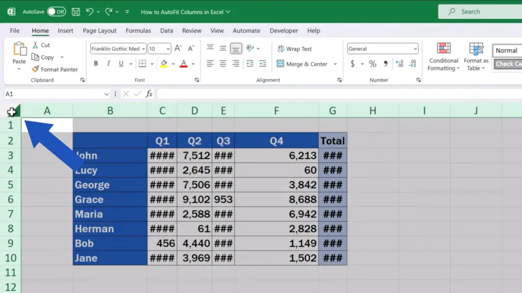
If a data table contains more columns, it’s easier to click into the top left-hand corner and select all columns in the sheet.

Either way works perfectly fine in Excel – choose whichever suits you best, the result after autofit will be the same.

Once selected, we set the cursor on a border of any two selected columns and see it change like this.

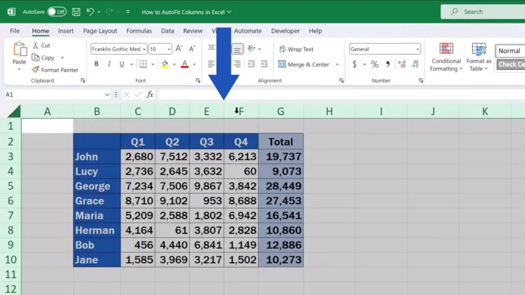
Now just do a quick double click with the left mouse button and here we go!

With all data visible, the width of the columns is the narrowest possible throughout the data table.

To learn more ways to amend column width, check out the video tutorial called How to Resize Multiple Columns in Excel (Three Most Common Ways). The link to the video is in the description below.

Don’t miss out a great opportunity to learn:

How to Switch Rows and Columns in Excel (the Easy Way)

If you found this tutorial helpful, give us a like and watch other tutorials by EasyClick Academy. Learn how to use Excel in a quick and easy way!

Is this your first time on EasyClick? We’ll be more than happy to welcome you in our online community. Hit that Subscribe button and join the EasyClickers!

Thanks for watching and I’ll see you in the next tutorial!