How to Add the Dollar Sign in Excel (Quick and Easy)

In this video tutorial, we’re going to have a look at how to add the dollar sign in Excel.

Quick and easy – let’s get started!

Contents hide

3 How to Set Decimal Places and Currency Symbol

How to Select Cells for Formatting

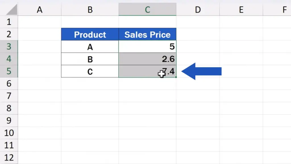
To add the dollar sign to numbers in an Excel spreadsheet, first let’s select all the numbers next to which we want to display the dollar sign.

How to Apply Currency Formatting

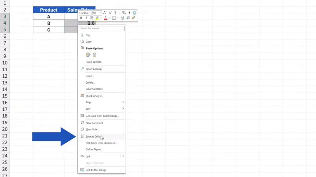
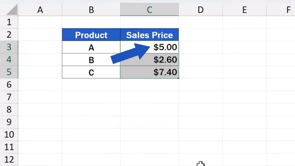
Here we’re going to add the sign next to the prices of the products A to C. Once selected, click on the right mouse button and choose ‘Format Cells’.

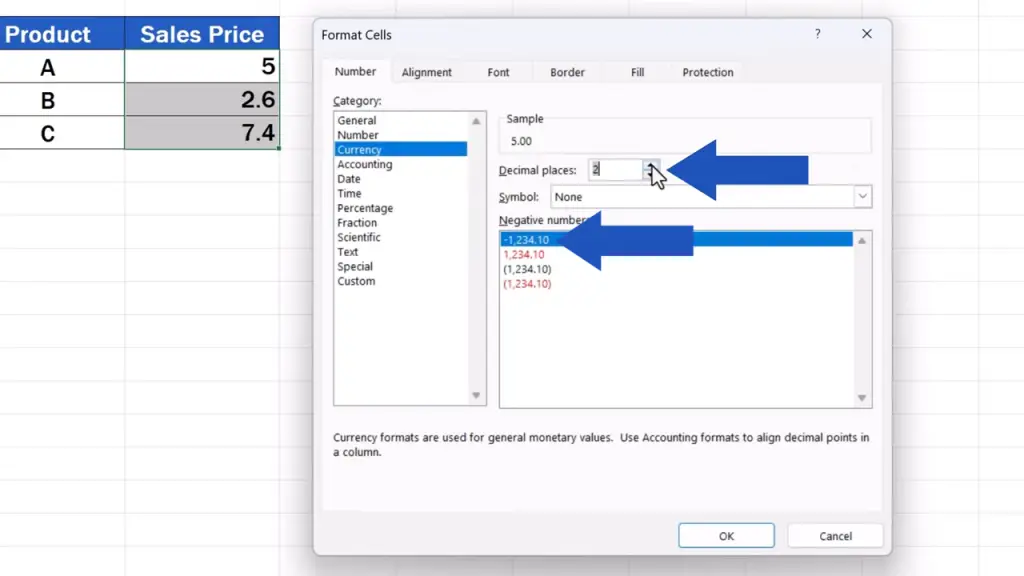
We’ve got this pop-up window here, where we look for ‘Category’ and there we select ‘Currency’.

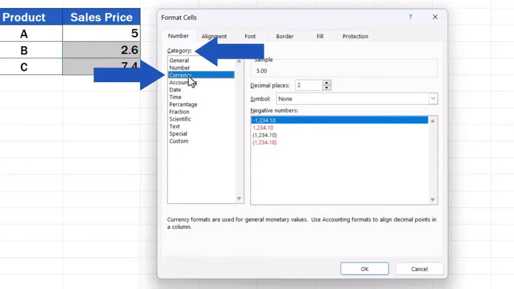
On the right you’ll see options like the number of decimal places to be displayed or a drop-down menu to pick the currency symbol to appear next to the numbers.

How to Set Decimal Places and Currency Symbol

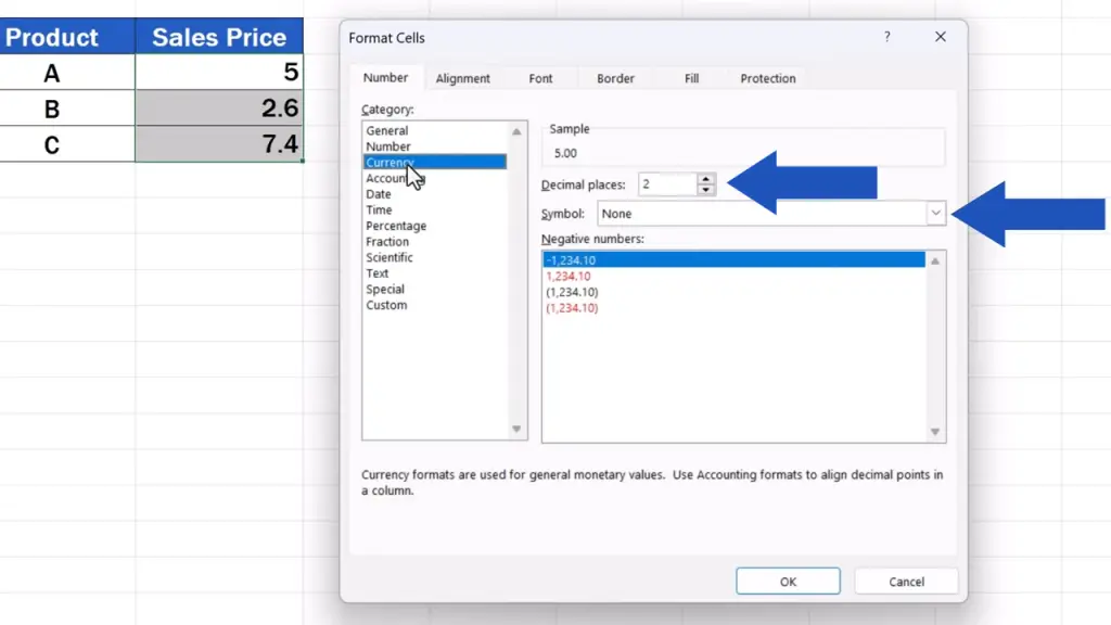
To set the number of decimal places to be displayed, use these arrows. We’ll leave it at 2 now.

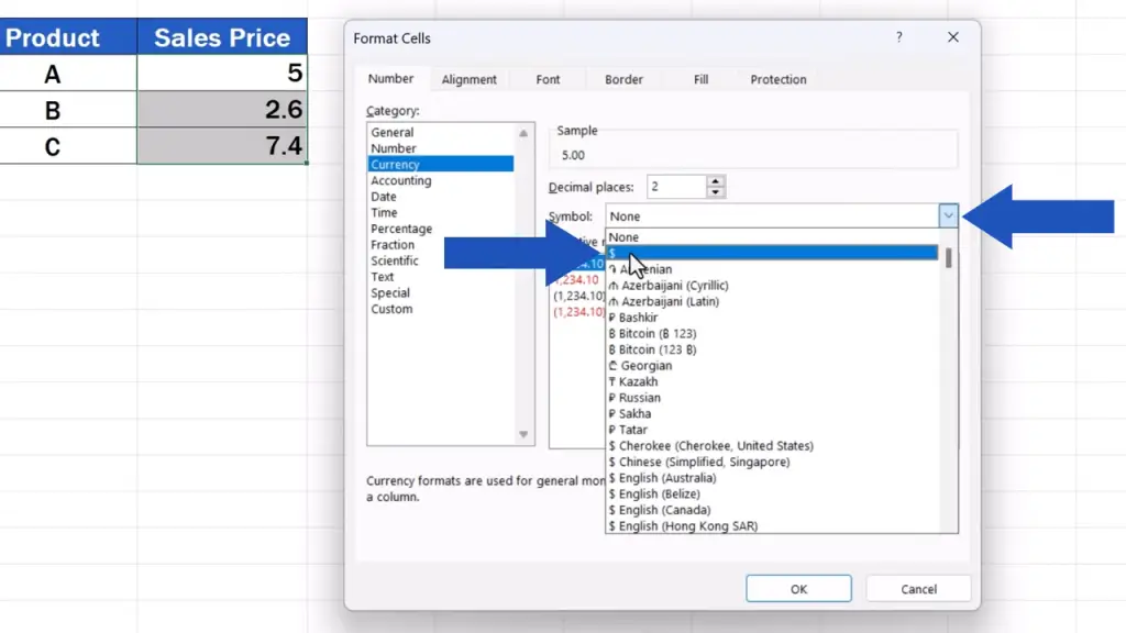
Then, in the ‘field Symbol’, open the drop-down menu and pick any currency symbol you need. In this case, we’ll go for the dollar sign, so we’ll click on the symbol of the dollar.

How to Finalize Formatting

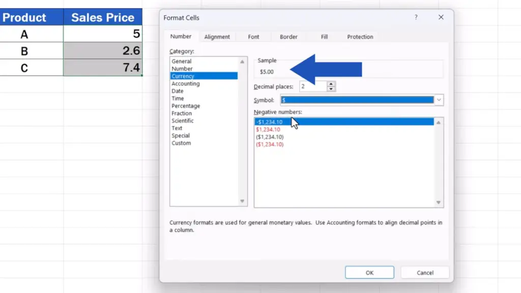
Up here, in the field ‘Sample’, we can see the preview of the numbers as they’ll appear with the current settings – with the currency symbol.

So, once everything’s been set press OK and that’s it!

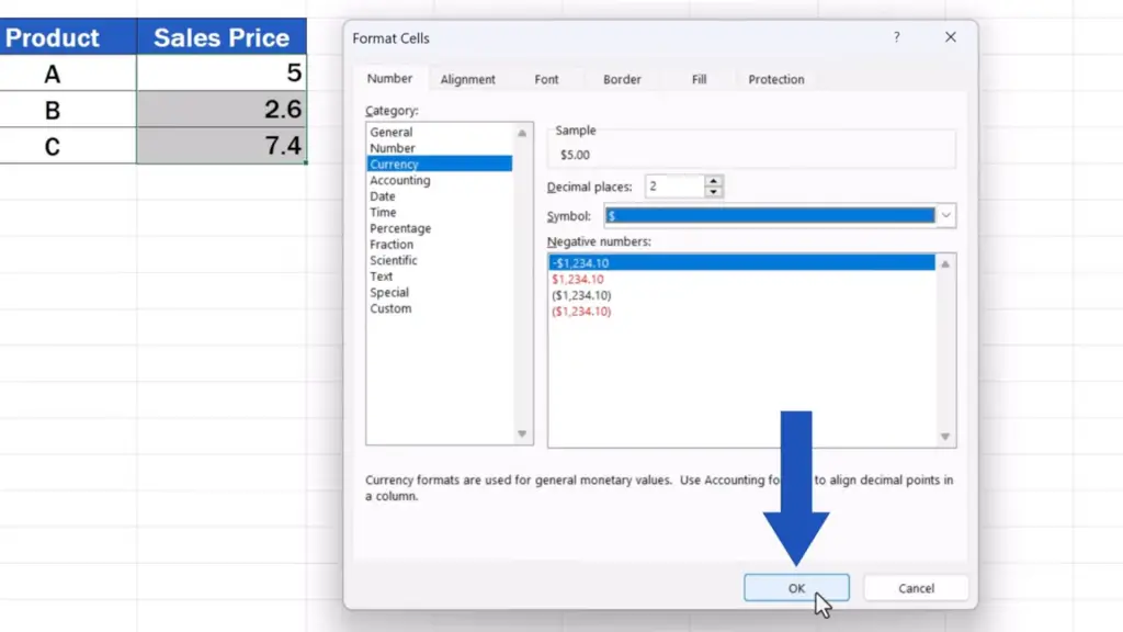
The dollar sign shows with all the numbers, which are displayed with two decimal places, just as we wanted.

Don’t miss out a great opportunity to learn:

If you found this tutorial helpful, give us a like and watch other tutorials by EasyClick Academy. Learn how to use Excel in a quick and easy way!

Is this your first time on EasyClick? We’ll be more than happy to welcome you in our online community. Hit that Subscribe button and join the EasyClickers!

Thanks for watching and I’ll see you in the next tutorial!