How to Remove Duplicates in Excel

In this short tutorial, I’ll guide you through some simple steps that will help you remove duplicates from a table. This can come quite handy, especially when comparing a huge amount of data, and it can save you a great deal of your precious time.

Ready?

See video tutorial and transcription below:

See this video on YouTube:
http://www.youtube.com/watch?v=g_NmTjzUHBA

In the last tutorial we learned how to find and highlight duplicates in a table.

Now you’ll see how you can remove them immediately from a table of any size. I’ll demonstrate it on a simple example, but this trick works with tables containing hundreds or thousands of data entries as well!

As you can see, rows 4 and 5 contain duplicated data.

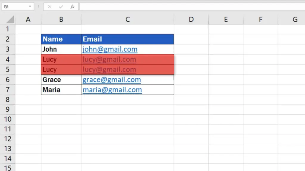
Our aim is to leave only one occurrence of this entry in the table and remove its duplicate. Now the question is how to achieve this.

How to Remove Duplicates in Exact Column in Excel

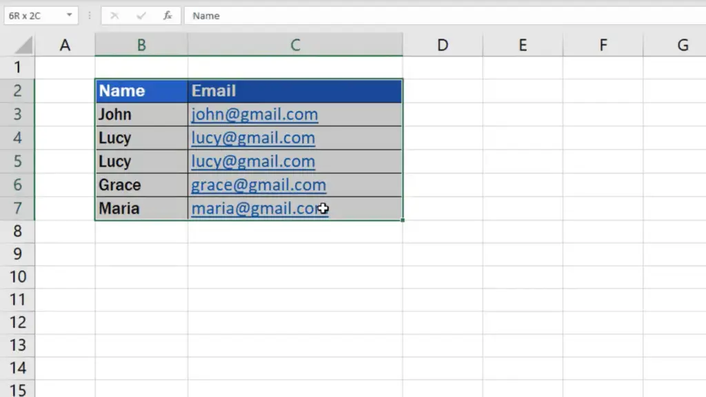
To start with, select the area in which you want Excel to find and remove duplicates. In this case, we’ll select the whole table.

Click on the Data tab, go to Data Tools, and choose the option Remove Duplicates.

A window will appear where you can choose in which columns you want Excel to find and remove duplicates. Usually, all columns are selected by default.

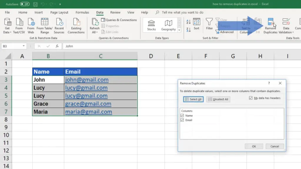
However, if we wanted to work only with the column ‘Email’, we could remove the tick from the box next to the column ‘Name’, which would mean that Excel would look for duplicates only in the column containing the email information. The column with names would be ignored.

This way you can choose in which columns you want to look for duplicates and which columns should be disregarded.

If the table happens to have headers, make sure to have the box ‘My data has headers’ ticked. Thanks to this option you will see specific names of the columns identified by their headers. Here we’ve got ‘Name’ and ‘Email’.

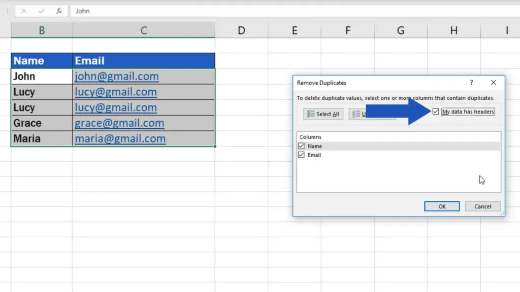
If we unselect this option, we can see only a generic column name marked with a letter. Like this…

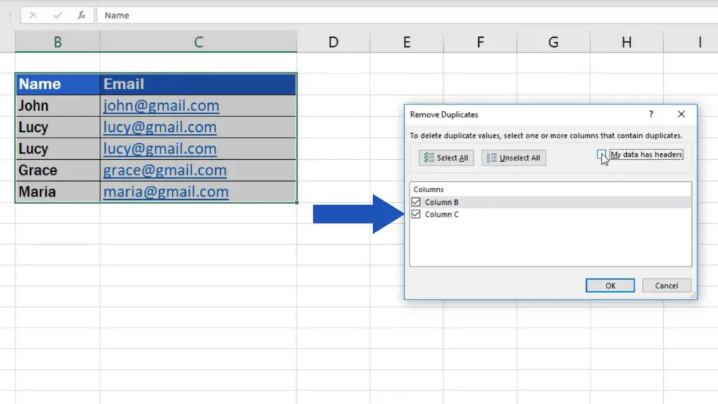
Let’s undo the changes and tick the option ‘My data has headers’ again and move on.

If everything has been set as you need, click on OK and Excel will remove all the duplicates from the table. It will also provide you with the information on how many duplicates have been found and removed, in a window similar to this one.

In our case, there was just one duplicated entry which I told you about at the beginning.

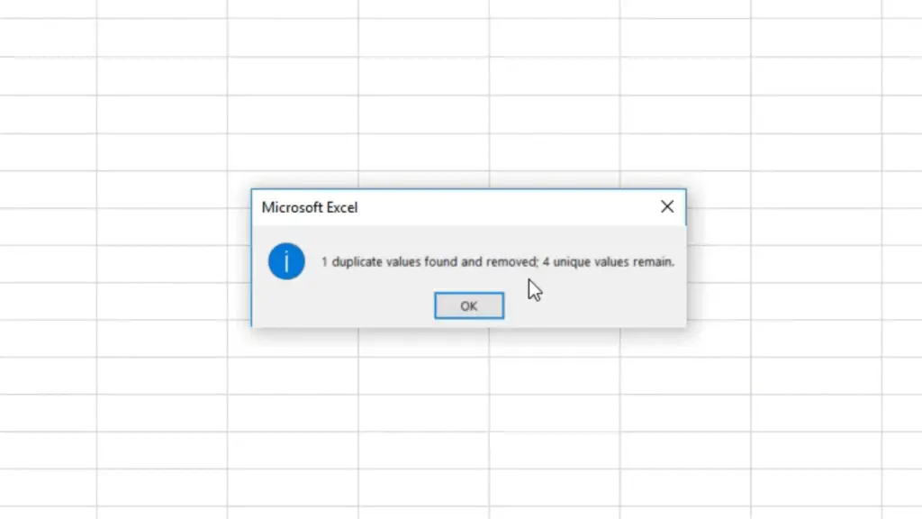
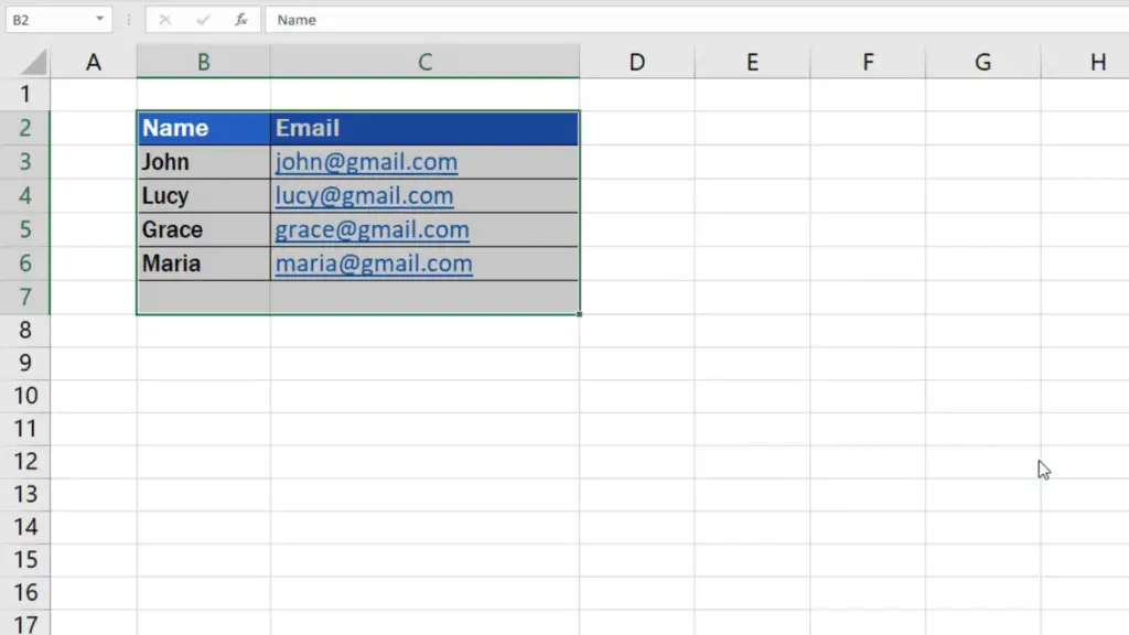
Click on OK. The table has now been cleared of duplicates. Only one occurrence for each data entry has been left.

Would you like to know How to Find Duplicates in Excel? Watch the next tutorial by EasyClick Academy!

If you’ve found this tutorial helpful, like us and subscribe to receive more videos from EasyClick Academy. Look at more tutorials that help you use Excel quick and easy!

See you in the next tutorial!